CONDOR, an new Parallel, Constrained
extension of Powell's UOBYQA algorithm.
Experimental results and comparison
with the DFO algorithm.
Frank Vanden Berghen, Hugues Bersini
IRIDIA, Université Libre de Bruxelles
50, av. Franklin Roosevelt
1050 Brussels, Belgium
Tel: +32 2 650 27 29, Fax: 32 2 650 27 15
fvandenb@iridia.ulb.ac.be, bersini@ulb.ac.be
Date: August 1, 2004
PDF version of this page is available
here.
Abstract:
This paper presents an algorithmic extension of Powell's UOBYQA algorithm
("
Unconstrained Optimization BY Quadratical Approximation"). We start
by summarizing the original algorithm of Powell and by presenting it in a more
comprehensible form. Thereafter, we report comparative numerical results between
UOBYQA, DFO and a parallel, constrained extension of UOBYQA that will be called
in the paper CONDOR ("
COnstrained, Non-linear, Direct, parallel Optimization
using trust Region method for high-computing load function"). The experimental
results are very encouraging and validate the approach. They open wide possibilities
in the field of noisy and high-computing-load objective functions optimization
(from two minutes to several days) like, for instance, industrial shape optimization
based on CFD (Computation Fluid Dynamic) codes or PDE (partial differential
equations) solvers. Finally, we present a new, easily comprehensible and fully
stand-alone implementation in C++ of the parallel algorithm.
Introduction
Powell's UOBYQA algorithm ([34] or [35]) is a new algorithm for unconstrained, direct optimization
that take into account the curvature of the objective function, leading to a high
convergence speed. UOBYQA is the direct successor of COBYLA [31]. Classical quasi-newton methods also use curvature information
([27,2,1,15,18]) but they need explicit gradient information, usually obtained
by finite difference. In the field of aerodynamical shape optimization, the objective
functions are based on expensive simulation of CFD (computation fluid dynamic)
codes (see [41,28,13,29,30]) or PDE (partial differential equations) solvers. For such
applications, choosing an appropriate step size for approximating the derivatives
by finite differences is quite delicate: function evaluation is expensive and
can be very noisy. For such type of application, finite difference quasi-newton
methods need to be avoided. Indeed, even if actual derivative information were
available, quasi-Newton methods might be a poor choice because adversely affected
by function inaccuracies (see [17]). Instead, direct optimization methods [16] are relatively insensitive to the noise. Unfortunately, they
usually require a great amount of function evaluations.
UOBYQA and CONDOR sample the search space, making evaluations in a way that reduces
the influence of the noise. They both construct a full quadratical model based
on Lagrange Interpolation technique [14,37,8,42,43,33]. The curvature information is obtained from the quadratical
model. This technique is less sensitive to the noise and leads to high quality
local quadratical models which directly guide the search to the nearest local
optimum. These quadratical models are built using the least number of evaluations
(possibly reusing old evaluations).
DFO [12,11] is an algorithm by A.R.Conn, K. Scheinberg and Ph.L. Toint.
It's very similar to UOBYQA and CONDOR. It has been specially designed for small
dimensional problems and high-computing-load objective functions. In other words,
it has been designed for the same kind of problems that CONDOR. DFO also uses
a model build by interpolation. It is using a Newton polynomial instead of a Lagrange
polynomial. When the DFO algorithm starts, it builds a linear model (using only
 evaluations of the objective function;
  is the dimension of the search space) and then directly uses this
simple model to guide the research into the space. In DFO, when a point is "too
far" from the current position, the model could be invalid and could
not represent correctly the local shape of the objective function. This "far point"
is rejected and replaced by a closer point. This operation unfortunately requires
an evaluation of the objective function. Thus, in some situation, it is preferable
to lower the degree of the polynomial which is used as local model (and drop the
"far" point), to avoid this evaluation. Therefore, DFO is using a polynomial of
degree oscillating between 1 and a "full" 2. In UOBYQA and CONDOR, we use the
Moré and Sorenson algorithm [26,9] for the computation of the trust region step. It is very
stable numerically and give very high precision results. On the other
hand, DFO uses a general purpose tool (NPSOL [20]) which gives high quality results but that cannot
be compared to the Moré and Sorenson algorithm when precision is critical.
An other critical difference between DFO and CONDOR/UOBYQA is the formula used
to update the local model. In DFO, the quadratical model built at each iteration
is not defined uniquely. For a unique quadratical model in variables one needs at least
is the dimension of the search space) and then directly uses this
simple model to guide the research into the space. In DFO, when a point is "too
far" from the current position, the model could be invalid and could
not represent correctly the local shape of the objective function. This "far point"
is rejected and replaced by a closer point. This operation unfortunately requires
an evaluation of the objective function. Thus, in some situation, it is preferable
to lower the degree of the polynomial which is used as local model (and drop the
"far" point), to avoid this evaluation. Therefore, DFO is using a polynomial of
degree oscillating between 1 and a "full" 2. In UOBYQA and CONDOR, we use the
Moré and Sorenson algorithm [26,9] for the computation of the trust region step. It is very
stable numerically and give very high precision results. On the other
hand, DFO uses a general purpose tool (NPSOL [20]) which gives high quality results but that cannot
be compared to the Moré and Sorenson algorithm when precision is critical.
An other critical difference between DFO and CONDOR/UOBYQA is the formula used
to update the local model. In DFO, the quadratical model built at each iteration
is not defined uniquely. For a unique quadratical model in variables one needs at least
 points and their function values. "In DFO,
models are often build using many fewer points and such models are not uniquely
defined" (citation from [11]). The strategy used inside DFO is to select the model with
the smallest Frobenius norm of the Hessian matrix. This update is highly numerically
instable [36]. Some recent research at this subject have maybe found a
solution [36] but this is still "work in progress". The model DFO is using
can thus be very inaccurate.
points and their function values. "In DFO,
models are often build using many fewer points and such models are not uniquely
defined" (citation from [11]). The strategy used inside DFO is to select the model with
the smallest Frobenius norm of the Hessian matrix. This update is highly numerically
instable [36]. Some recent research at this subject have maybe found a
solution [36] but this is still "work in progress". The model DFO is using
can thus be very inaccurate.
In contrast to UOBYQA and CONDOR, DFO uses linear or quadratical models to guide
the search, thus requiring less function evaluations to build the local models.
Based on our experimental results, we surprisingly discovered that CONDOR used
less function evaluations than DFO to reach an optimum point, despite the fact
that the cost to build a local model is higher (see section 5 presenting numerical
results). This is most certainly due to an heuristic (see section 5.1
at this subject) used inside UOBYQA and CONDOR which allows to build quadratical
models at very "low price".
The algorithm used inside UOBYQA is thus a good choice to reduce the number of
function evaluations in the presence of noisy and high computing load objective
functions. Since description of this algorithm in the literature is hard to find
and rather unclear, a first objective of the paper is to provide an updated and
more accessible version of it.
When concerned with CPU time to reach the local optimum, computer parallelization
of the function evaluations is always an interesting road to pursue. Indeed, PDS
(Parallel direct search) largely exploits this parallelization to reduce the optimization
time. We take a similar road by proposing an extension of the original UOBYQA
that can use several CPU's in parallel: CONDOR. Our experimental results show
that this addition makes CONDOR the fastest available algorithm for noisy, high
computing load objective functions (fastest in terms of number of function evaluations).
In substance, this paper proposes a new, simpler and clearer, parallel implementation
in C++ of UOBYQA: the CONDOR optimizer. A version of CONDOR allowing constraints
is discussed in [40]. The paper is structured in the following way:
- Section 1: The introduction.
- Section 2: Basic description of the UOBYQA algorithm with hints to
possible parallelization.
- Section 3: New, more in depth, comprehensible presentation of UOBYQA
with a more precise description of the parallel extension.
- Section 4: In depth description of this parallel extension.
- Section 5: Experimental results: comparison between CONDOR, the original
Powell's UOBYQA, DFO, LANCELOT, COBYLA, PDS.
- Section 5: How to get the code and conclusions.
Let be the dimension of the search space. Let  be the objective function to minimize. We want to find
 which satisfies:
 |
(1) |
In the following algorithm,  is the usual trust region radius. We do not allow to increase because this would necessitate expensive decrease
later. We will introduce
is the usual trust region radius. We do not allow to increase because this would necessitate expensive decrease
later. We will introduce  , another trust region radius that satisfies
 . The advantage of is to allow the length of the steps to exceed and to increase the efficiency of the algorithm.
Let  be the starting point of the algorithm. Let
 and
and
 be the initial and final value of the trust region radius
.
be the initial and final value of the trust region radius
.
Basically, Powell's UOBYQA algorithm does the following (for a more detailed
explanation, see section 3 or [34]):
- Create an interpolation polynomial
 of degree 2 which interpolates the objective function around
. All the points in the interpolation set
of degree 2 which interpolates the objective function around
. All the points in the interpolation set
 (used to build
  ) are separated by a distance of approximatively
. Set
) are separated by a distance of approximatively
. Set  the best point of the objective function known so far.
Set
the best point of the objective function known so far.
Set
 . In the following algorithm,
  is the quadratical approximation of around
  :
:
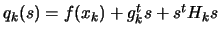 where
where  is an approximation of the gradient of evaluated at and
  is an approximation of the Hessian matrix of evaluated at .
- Set

- Inner loop: solve the problem for a given precision of
 .
.
-
- Solve
 subject to
 .
.
- If
 , then break and go to step 3(b)
because, in order to do such a small step, we need to be sure that
the model is valid.
, then break and go to step 3(b)
because, in order to do such a small step, we need to be sure that
the model is valid.
- Evaluate the function at the new position
 . Update (like described in next section, 4(a)viii. to 4(a)x.
) the trust region radius
. Update (like described in next section, 4(a)viii. to 4(a)x.
) the trust region radius  and the current best point using classical trust region technique. Include the new inside the interpolation set
. Update to interpolate on the new
.
and the current best point using classical trust region technique. Include the new inside the interpolation set
. Update to interpolate on the new
.
- If some progress has been achieved (for example,
 or there was a reduction
 ), increment
  and go back to step 3(a)i, otherwise continue.
- Test the validity of
 in
in

 , like described in [34].
- Model is invalid:
Improve the quality of the model : Remove the worst point of the interpolation set
and replace it (one evaluation required!) with a new point
 such that:
 and the precision of is substantially increased.
- Model is valid:
If
 go back to step 3(a), otherwise continue.
- Reduce since the optimization steps
 are becoming very small, the accuracy needs to be raised.
- If
 stop, otherwise increment k and go back to step 2.
Basically, is the distance (Euclidian distance) which separates the points
where the function is sampled. When the iterations are unsuccessful, the trust
region radius decreases, preventing the algorithm to achieve more progress.
At this point, loop 3(a)i to 3(a)iv is exited and a function evaluation is required
to increase the quality of the model (step 3(b)). When the algorithm comes close
to an optimum, the step size becomes small. Thus, the inner loop (steps 3(a)i.
to 3(a)iv.) is usually exited from step 3(a)ii, allowing to skip step 3(b) (hoping
the model is valid), and directly reducing in step 4.
The most inner loop (steps 3(a)i. to 3(a)iv.) tries to get from good search directions without doing any extra evaluation to
maintain the quality of (The evaluations that are performed on step 3(a)i) have another
goal). Only inside step 3(b), evaluations are performed to increase this quality
(called a "model step") and only at the condition that the model has been proven
to be invalid (to spare evaluations!).
Notice the update mechanism of in step 4. This update occurs only when the model has been validated
in the trust region
(when the loop 3(a) to 3(b) is exited). The function cannot
be sampled at point too close to the current point without being assured that the model is valid in
. This mechanism protects us against noise.
The different evaluations of are used to:
- (a)
- guide the search to the minimum of (see inner loop in the steps 3(a)i. to 3(a)iv.). To guide the
search, the information gathered until now and available in is exploited.
- (b)
- increase the quality of the approximator (see step 3(b)). To avoid the degeneration of , the search space needs to be additionally explored.
(a) and (b) are antagonist objectives like frequently encountered in the exploitation/exploration
paradigm. The main idea of the parallelization of the algorithm is to perform
the exploration on distributed CPU's. Consequently, the algorithm will
have better models of available and choose better
search direction, leading to a faster convergence.
UOBYQA and CONDOR are inside the class of algorithm which are proven to be globally
convergent to a local (maybe global) optimum: They are both using conditional
models as described in [12,8].
The UOBYQA algorithm in depth
We will now detail the UOBYQA algorithm [34] and a part of its parallel extension. As a result of this
parallel extension, the points 3, 4(a)i, 4(b), 9 constitute an original contribution
of the authors. When only one CPU is available, these points are simply skipped.
The point 4(a)v is also original and has been added to make the algorithm more
robust against noise in the evaluation of the objective function. These points
will be detailed in the next section. The other points of the algorithm belong
to the original UOBYQA.
Let  and
and  , be the absolute and relative error on the evaluation of the
objective function. These constants are given by the user. By default, they are
null.
, be the absolute and relative error on the evaluation of the
objective function. These constants are given by the user. By default, they are
null.
- Set
 ,
,
 and generate a first interpolation set
 around (with
 ). This set is "poised", meaning that the Vandermonde
determinant of
is non-null (see [14,37]). The set
is generated using the algorithm described in [34].
). This set is "poised", meaning that the Vandermonde
determinant of
is non-null (see [14,37]). The set
is generated using the algorithm described in [34].
- In what follows, the index is always the index of the best point of the set
. The points
in
will be noted in bold with parenthesis around their
subscript. Let
 . Set
. Set
 . Apply a translation of
 to all the dataset
 and generate
the quadratical polynomial , which intercepts all the points in the dataset
. The translation is achieved to increase the quality of
the interpolation. is built using Multivariate Lagrange Interpolation. It means
that
and generate
the quadratical polynomial , which intercepts all the points in the dataset
. The translation is achieved to increase the quality of
the interpolation. is built using Multivariate Lagrange Interpolation. It means
that
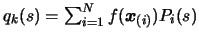 where the
  are the Lagrange polynomials associated to the dataset
. The have the following property:
are the Lagrange polynomials associated to the dataset
. The have the following property:
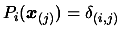 where
where
 is the Kronecker delta (see [14,37] about multivariate Lagrange polynomial interpolation). The
complete procedure is given in [34].
is the Kronecker delta (see [14,37] about multivariate Lagrange polynomial interpolation). The
complete procedure is given in [34].
- Parallel extension: Start the "parallel computations" on the different
computer nodes. See next section for more details.
-
-
- Parallel extension: Check the results of the parallel computation
and use them to increase the quality of . See next section for more details.
- Calculate the "Trust region step"
 : is the solution of:
This is a quadratic program with a non-linear constraint. It's solved
using Moré and Sorenson algorithm (see [26,9]). The original implementation of the UOBYQA algorithm uses
a special tri-diagonal decomposition of the Hessian to obtain high
speed (see [32]). CONDOR uses a direct, simpler, implementation of the Moré
and Sorenson algorithm.
: is the solution of:
This is a quadratic program with a non-linear constraint. It's solved
using Moré and Sorenson algorithm (see [26,9]). The original implementation of the UOBYQA algorithm uses
a special tri-diagonal decomposition of the Hessian to obtain high
speed (see [32]). CONDOR uses a direct, simpler, implementation of the Moré
and Sorenson algorithm.
- If
 , then break and go to
step 4(b): the model needs to be validated before doing such a small
step.
, then break and go to
step 4(b): the model needs to be validated before doing such a small
step.
- Let
 , the
predicted reduction of the objective function.
, the
predicted reduction of the objective function.
- One original addition to the algorithm is the following:
Let
![$ noise: = \frac{1}{2} \max [ noise_a*(1+noise_r), noise_r
\vert f(\boldsymbol{x}_{(k)})\vert ]$](img60.png) .
.
If  , break and go to step 4(b).
- Evaluate the objective function at point
 . The result of this evaluation is stored
in the variable
. The result of this evaluation is stored
in the variable  .
.
- Compute the agreement
 between and the model :
- Update the trust region radius :
If
 , set
, set
 .
.
- Store
 inside the interpolation dataset
. To do so, first, choose the worst point
inside the interpolation dataset
. To do so, first, choose the worst point
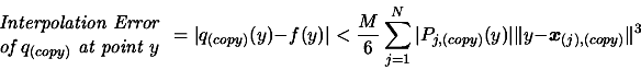
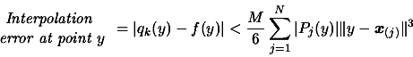
 of the dataset (The exact, detailed algorithm,
is given in [34]). This is the point which gives the highest contribution
to following bound on the interpolation error [33]:
of the dataset (The exact, detailed algorithm,
is given in [34]). This is the point which gives the highest contribution
to following bound on the interpolation error [33]:
 |
(2) |
Where  is a bound on the third derivative of :
 where
where
 and
and  , and where
  are the Lagrange Polynomials used to construct
  .(see [14,37] about multivariate Lagrange polynomial interpolation).
Secondly, replace the point
by
and recalculate the new quadratic which interpolates the new dataset.
 The
The  is
is
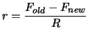
- Update the index of the best point in the dataset.
Set
![$ F_{new} := \min [ F_{old}, F_{new} ]$](img81.png) .
.
- Update the value (the bound on the third derivative of ) using:
![$\displaystyle M_{new}= \max \bigg[ M_{old}, \frac{\vert
q_k(x)-f(x) \vert }{ \...
...sum_{j=1}^N \vert P_j(x) \vert \Vert x -
\boldsymbol{x}_{(j)} \Vert^3 } \bigg]$](img82.png) |
(3) |
- If there is an improvement in the quality of the solution (
 ) OR if
 OR if
OR if
 then go back to point 4(a)i, otherwise, continue.
- Parallel extension: Check the results of the parallel computation
and use them to increase the quality of . See next section for more details.
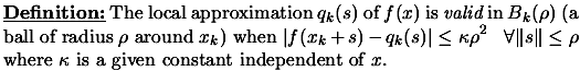
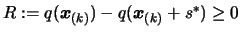
- The validity of our model in
 , a ball of radius around
 now needs to be checked based on equations (6)
and (7).
now needs to be checked based on equations (6)
and (7).
- Model is invalid:
Improve the quality of our model . This is called a "model improvement step". Remove the worst point
 of the dataset and replace it by a better point.
This better point is computed using an algorithm described in [34]. If a new function evaluation has been made, the value of
must also be updated. Possibly, an update of the index of the best point in the dataset
and
of the dataset and replace it by a better point.
This better point is computed using an algorithm described in [34]. If a new function evaluation has been made, the value of
must also be updated. Possibly, an update of the index of the best point in the dataset
and  is required. Once this is finished, go back to step 4(a).
- Model is valid:
If
 go back to step 4(a), otherwise continue.
- If
, the algorithm is nearly finished. Go to step 8, otherwise
continue to the next step.
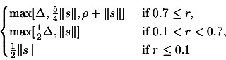
- Update of trust region radius .
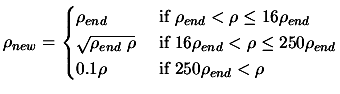 |
(4) |
Set
![$ \displaystyle \Delta:=\max[\frac{\rho}{2}, \rho_{new}]$](img92.png) . Set
. Set
 .
.
- Set
 . Apply a translation
of
. Apply a translation
of
 to , to the set of Newton polynomials
  which defines and to the whole dataset
. Go back
to step 4.
which defines and to the whole dataset
. Go back
to step 4.
- The iterations are now complete but one more value of may be required before termination. Indeed, it is known from step
4(a)iii and step 4(a)v of the algorithm that the value of
 could not have been computed.
Compute
could not have been computed.
Compute
 .
.
- if
, the solution of the optimization problem is
 and the value of
  at this point is .
- if
 , the solution of the optimization problem is
 and the value of at this point is .
- Parallel extension: Stop the parallel computations if necessary.
The aim of the parallelization is to evaluate at positions which could substantially increase the quality of
the approximator . The way to choose such positions is explained in section 4.
The parallel extension of UOBYQA
We will use a client-server approach. The main node, the server, will run two
concurrent processes:
- The main process on the main computer is the classical non-parallelized
version of the algorithm, described in the previous section. There is an exchange
of information with the second/parallel process on steps 4(a)i and 4(b) of
the original algorithm.
- The goal of the second/parallel process on the main computer is to
increase the quality of the model by using client computers to sample at specific interpolation sites.
In an ideal scenario:
- The main process will always stay inside the most inner loop 4(a)i
to 4(a)xii. Hoping that the evaluation on the client computers always provide
a valid local model , progress will constantly be achieved.
- The main process exits the inner loop at step 4(a)iii: Near an optimum,
the model is ideally valid and can be decreased.
The client nodes are performing the following:
- Wait to receive from the second/parallel process on the server a sampling
site (a point).
- Evaluate the objective function at this site and return immediately the
result to the server.
- Go to step 1.
Several strategies have been tried to select good sampling sites. We describe
here the most promising one. The second/parallel task is the following:
- A.
- Make a local copy
 of (and of the associated Lagrange Polynomials
  )
)
- B.
- Make a local copy

 of the dataset
.
of the dataset
.
- C.
- Find the index
 of the point inside
the further away from
.
of the point inside
the further away from
.
- D.
- Replace
by a better point
 which will increase the quality of the approximation
of . The computation of this point is detailed below.
which will increase the quality of the approximation
of . The computation of this point is detailed below.
- E.
- Ask for an evaluation of the objective function at point
using a free client computer to perform the
evaluation. If there is still a client idle, go back to step C.
- F.
- Wait for a node to finish its evaluation of the objective function . Most of the time, the second/parallel task will be blocked here
without consuming any resources.
- G.
- Update
 using the newly received evaluation. Update
. go to step C.
using the newly received evaluation. Update
. go to step C.
In the parallel/second process we are always working on a copy of ,
and
 to avoid any side effect with the main process which
is guiding the search. The communication and exchange of information between these
two processes are done only at steps 4(a)i and 4(b) of the main process
described in the previous section. Each time the main process checks the results
of the parallel computations the following is done:
to avoid any side effect with the main process which
is guiding the search. The communication and exchange of information between these
two processes are done only at steps 4(a)i and 4(b) of the main process
described in the previous section. Each time the main process checks the results
of the parallel computations the following is done:
- i.
- Wait for the parallel/second task to enter the step F described
above and block the parallel task inside this step F for the time needed
to perform the points ii and iii below.
- ii.
- Update of using all the points calculated in parallel, discarding the
points that are too far away from
(at a distance greater than )(The points are inside
). This update is performed using technique described in [34]. We will possibly have to update the index of the best point in the dataset
and .
- iii.
- Perform operations described in point A & B of the parallel/second
task algorithm above: "Copy
from .
Copy
from
".
In step D. of the parallel algorithm, we must find a point which increase
substantially the quality of the local approximation
of . In the following, the discovery of this better point is explained.
The equation (2) is used. We will restate it here for
clarity:
where and
 have the same signification as for equation (2).
Note also that we are working on a copy of
have the same signification as for equation (2).
Note also that we are working on a copy of
 and
and  . In the remaining of the current section, we will drop the subscript for easier notation.
This equation has a special structure. The contribution to the interpolation error
of the point
to be dropped is easily separable from the contribution
of the other points of the dataset
, it is:
error due to  |
(5) |
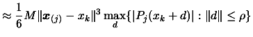
If  is inside the ball of radius around ( is the best point found until now in the second/parallel task),
then an upper bound of equation (5) can be found:
is inside the ball of radius around ( is the best point found until now in the second/parallel task),
then an upper bound of equation (5) can be found:
We are ignoring the dependence of the other Newton polynomials in the hope of
finding a useful technique and cheap to implement.
is thus replaced in
 by
by  where
where  is the solution of the following problem:
The algorithm used to solve this problem is described in [34].
Numerical Results
Results on one CPU
We will now compare CONDOR with UOBYQA [34], DFO [12,11], PDS [16], LANCELOT [7] and COBYLA [31] on a part of the Hock and Schittkowski test set [23]. The test functions and the starting points are extracted
from SIF files obtained from CUTEr, a standard test problem database for non-linear
optimization (see [22]). We are thus in perfect standard conditions. The tests problems
are arbitrary and have been chosen by A.R.Conn, K. Scheinberg and Ph.L. Toint.
to test their DFO algorithm. The performances of DFO are thus expected to be,
at least, good. We list the number of function evaluations that each algorithm
took to solve the problem. We also list the final function values that each algorithm
achieved. We do not list the CPU time, since it is not relevant in our context.
The "*" indicates that an algorithm terminated early because the limit on the
number of iterations was reached. The default values for all the parameters of
each algorithm is used. The stopping tolerance of DFO was set to  , for the other algorithms the tolerance was set to appropriate
comparable default values. The comparison between the algorithms is based on the
number of function evaluations needed to reach the SAME precision. For the most
fair comparison with DFO, the stopping criteria (
) of CONDOR has been chosen so that CONDOR is always stopping
with a little more precision on the result than DFO. This precision is some time
insufficient to reach the true optima of the objective function. In particular,
in the case of the problems GROWTHLS and HEART6LS, the CONDOR algorithm can find
a better optimum after some more evaluations (for a smaller
). All algorithms were implemented in Fortran 77 in double
precision except COBYLA which is implemented in Fortran 77 in single precision
and CONDOR which is written in C++ (in double precision). The trust region minimization
subproblem of the DFO algorithm is solved by NPSOL [20], a fortran 77 non-linear optimization package that uses an
SQP approach. For CONDOR, the number in parenthesis indicates the number of function
evaluation needed to reach the optimum without being assured that the value found
is the real optimum of the function. For example, for the WATSON problem, we find
the optimum after (580) evaluations. CONDOR still continues to sample the objective
function, searching for a better point. It's loosing 87 evaluations in this search.
The total number of evaluation (reported in the first column) is thus 580+87=667.
, for the other algorithms the tolerance was set to appropriate
comparable default values. The comparison between the algorithms is based on the
number of function evaluations needed to reach the SAME precision. For the most
fair comparison with DFO, the stopping criteria (
) of CONDOR has been chosen so that CONDOR is always stopping
with a little more precision on the result than DFO. This precision is some time
insufficient to reach the true optima of the objective function. In particular,
in the case of the problems GROWTHLS and HEART6LS, the CONDOR algorithm can find
a better optimum after some more evaluations (for a smaller
). All algorithms were implemented in Fortran 77 in double
precision except COBYLA which is implemented in Fortran 77 in single precision
and CONDOR which is written in C++ (in double precision). The trust region minimization
subproblem of the DFO algorithm is solved by NPSOL [20], a fortran 77 non-linear optimization package that uses an
SQP approach. For CONDOR, the number in parenthesis indicates the number of function
evaluation needed to reach the optimum without being assured that the value found
is the real optimum of the function. For example, for the WATSON problem, we find
the optimum after (580) evaluations. CONDOR still continues to sample the objective
function, searching for a better point. It's loosing 87 evaluations in this search.
The total number of evaluation (reported in the first column) is thus 580+87=667.
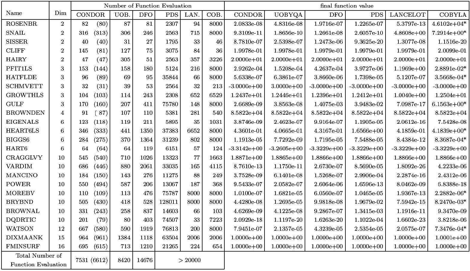
CONDOR and UOBYQA are both based on the same algorithm and have nearly the same
behavior.
PDS stands for "Parallel Direct Search" [16]. The number of function evaluations is high and so the method
doesn't seem to be very attractive. On the other hand, these evaluations can be
performed on several CPU's reducing considerably the computation time.
Lancelot [7] is a code for large scale optimization when the number of
variable is  and the objective function is easy to evaluate (less than
 .). Its model is build using finite differences and BFGS update.
This algorithm has not been design for the kind of application we are interested
in and is thus performing accordingly.
.). Its model is build using finite differences and BFGS update.
This algorithm has not been design for the kind of application we are interested
in and is thus performing accordingly.
COBYLA [31] stands for "Constrained Optimization by Linear Approximation"
by Powell. It is, once again, a code designed for large scale optimization. It
is a derivative free method, which uses linear polynomial interpolation of the
objective function.
DFO [12,11] is an algorithm by A.R.Conn, K. Scheinberg and Ph.L. Toint.
It has already been described in section 1. In CONDOR
and in UOBYQA the validity of the model is checked using two equations:
 |
(6) |
 |
(7) |
using notation of section 3. See [34] to know how to compute  . The first equation (6) is also used
in DFO. The second equation (7) (which is similar to equation
(2)) is NOT used in DFO. This last equation allows us
to "keep far points" inside the model, still being assured that it is valid. It
allows us to have a "full" polynomial of second degree for a "cheap price". The
DFO algorithm cannot use equation 7 to check the validity
of its model because the variable (which is computed in UOBYQA and in CONDOR as a by-product
of the computation of the "Moré and Sorenson Trust Region Step") is not cheaply
available. In DFO, the trust region step is calculated using an external tool:
NPSOL [20]. is difficult to obtain and is not used.
. The first equation (6) is also used
in DFO. The second equation (7) (which is similar to equation
(2)) is NOT used in DFO. This last equation allows us
to "keep far points" inside the model, still being assured that it is valid. It
allows us to have a "full" polynomial of second degree for a "cheap price". The
DFO algorithm cannot use equation 7 to check the validity
of its model because the variable (which is computed in UOBYQA and in CONDOR as a by-product
of the computation of the "Moré and Sorenson Trust Region Step") is not cheaply
available. In DFO, the trust region step is calculated using an external tool:
NPSOL [20]. is difficult to obtain and is not used.
UOBYQA and CONDOR are always using a full quadratic model. This enables us to
compute Newton's steps. The Newton's steps have a proven quadratical convergence
speed [15]. Unfortunately, some evaluations of the objective function
are lost to build the quadratical model. So, we only obtain *near* quadratic speed
of convergence. We have Q-superlinear convergence (see original paper of Powell
[34]). (In fact the convergence speed is often directly proportional
to the quality of the approximation of the real Hessian matrix of ). Usually, the price (in terms of number of function evaluations)
to construct a good quadratical model is very high but using equation (7),
UOBYQA and CONDOR are able to use very few function evaluations to update the
local quadratical model.
When the dimension of the search space is greater than 25, the time needed to
start, building the first quadratic, is so important ( evaluations) that DFO may becomes attractive again. Especially, if
you don't want the optimum of the function but only a small improvement in a small
time. If several CPU's are available, then CONDOR once again imposes itself. The
function evaluations needed to build the first quadratic are parallelized on all
the CPU's without any loss of efficiency when the number of CPU increases (the
maximum number of CPU is
evaluations) that DFO may becomes attractive again. Especially, if
you don't want the optimum of the function but only a small improvement in a small
time. If several CPU's are available, then CONDOR once again imposes itself. The
function evaluations needed to build the first quadratic are parallelized on all
the CPU's without any loss of efficiency when the number of CPU increases (the
maximum number of CPU is  ). This first construction phase has a great parallel efficiency,
as opposed to the rest of the optimization algorithm where the efficiency becomes
soon very low (with the number of CPU increasing). In contrast to CONDOR, the
DFO algorithm has a very short initialization phase and a long research phase.
This last phase can't be parallelized very well. Thus, when the number of CPU's
is high, the most promising algorithm for parallelization is CONDOR. A parallel
version of CONDOR has been implemented. Very encouraging experimental results
on the parallel code are given in the next section.
). This first construction phase has a great parallel efficiency,
as opposed to the rest of the optimization algorithm where the efficiency becomes
soon very low (with the number of CPU increasing). In contrast to CONDOR, the
DFO algorithm has a very short initialization phase and a long research phase.
This last phase can't be parallelized very well. Thus, when the number of CPU's
is high, the most promising algorithm for parallelization is CONDOR. A parallel
version of CONDOR has been implemented. Very encouraging experimental results
on the parallel code are given in the next section.
When the local model is not convex, no second order convergence proof (see [10]) is available. It means that, when using a linear model,
the optimization process can prematurely stop. This phenomenon *can* occur with
DFO which uses from time to time a simple linear model. CONDOR is very robust
and always converges to a local optimum (extensive numerical tests have been made
[40]).
Parallel results
We are using the same test conditions as for the previous section (standard objective
functions with standard starting points).
Since the objective function is assumed to be time-expensive to evaluate, we can
neglect the time spent inside the optimizer and inside the network transmissions.
To be able to make this last assumption (negligible network transmissions times),
a wait loop of 1 second is embedded inside the code used to evaluate the objective
function (only 1 second: to be in the worst case possible).
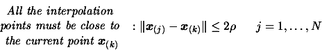
Figure 2: Improvement due to parallelism
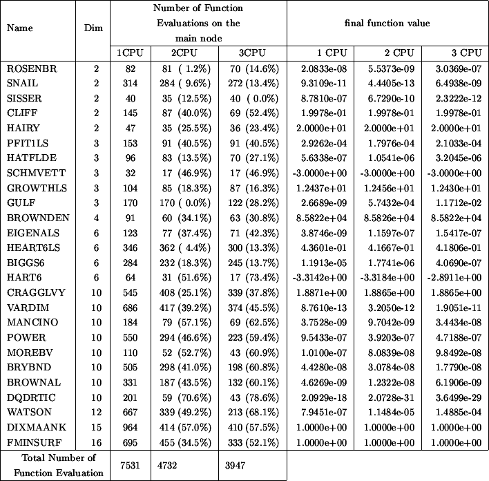 |
Table 2 indicates the number of function evaluations performed
on the master CPU (to obtain approximatively the total number of function evaluations
cumulated over the master and all the slaves, multiply the given number on the
list by the number of CPU's). The CPU time is thus directly proportional to the
numbers listed in columns 3 to 5 of the table 2.
Suppose a function evaluation takes 1 hour. The parallel/second process on the
main computer has asked 59 minutes ago to a client to perform one such evaluation.
We are at step 4(a)i of the main algorithm. We see that there are no new evaluation
available from the client computers. Should we go directly to step 4(a)ii and
use later this new information, or wait 1 minute? The response is clear: wait
a little. This bad situation occurs very often in our test examples since every
function evaluation takes exactly the same time (1 second). But what's the best
strategy when the objective function is computing, randomly, from 40 to 80 minutes
at each evaluation (this is for instance the case for objective functions which
are calculated using CFD techniques)? The response is still to investigate. Currently,
the implemented strategy is: never wait. Despite, this simple strategy, the current
algorithm gives already some non-negligible improvements.
We will assume that objective functions derived from CFD codes have usually a
simple shape but are subject to high-frequency, low amplitude noise. This noise
prevents us to use simple finite-differences gradient-based algorithms. Finite-difference
is highly sensitive to the noise. Simple Finite-difference quasi-Newton algorithms
behave so badly because of the noise, that most researchers choose to use optimization
techniques based on GA,NN,... [41,13,29,30]. The poor performances of finite-differences gradient-based
algorithms are either due to the difficulty in choosing finite-difference step
sizes for such a rough function, or the often cited tendency of derivative-based
methods to converge to a local optimum [4]. Gradient-based algorithms can still be applied but a clever
way to retrieve the derivative information must be used. One such algorithm is
DIRECT [21,24,5] which is using a technique called implicit filtering. This
algorithm makes the same assumption about the noise (low amplitude, high frequency)
and has been successful in many cases [5,6,38]. For example, this optimizer has been used to optimize the
cost of fuel and/or electric power for the compressor stations in a gas pipeline
network [6]. This is a two-design-variables optimization problem. You
can see in the right of figure 5 a plot of the
objective function. Notice the simple shape of the objective function and the
small amplitude, high frequency noise. Another family of optimizers is based on
interpolation techniques. DFO, UOBYQA and CONDOR belongs to this last family.
DFO has been used to optimize (minimize) a measure of the vibration of a helicopter
rotor blade [4]. This problem is part of the Boeing problems set [3]. The blade are characterized by 31 design variables. CONDOR
will soon be used in industry on a daily basis to optimize the shape of the blade
of a centrifugal impeller [28]. All these problems (gas pipeline, rotor blade and impeller
blade) have an objective function based on CFD code and are both solved using
gradient-based techniques. In particular, on the rotor blade design, a comparative
study between DFO and other approaches like GA, NN,... has demonstrated the clear
superiority of gradient-based techniques approach combined with interpolation
techniques [4].
We will now illustrate the performances of CONDOR in two simple cases which have
sensibly the same characteristics as the objective functions encountered in optimization
based on CFD codes. The functions, the amplitude of the artificial noise applied
to the objective functions (uniform noise distribution) and all the parameters
of the tests are summarized in table 5.3. In this table "NFE"
stands for Number of Function Evaluations. Each columns represents 50
runs of the optimizer.
Figure 3: Noisy optimization.
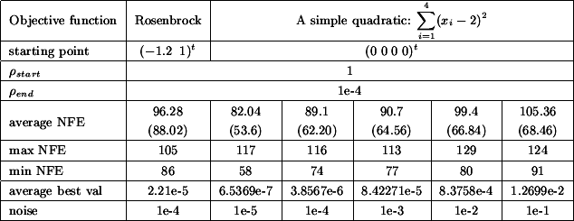 |
Figure 4: On the left: A typical run for the optimization
of the noisy Rosenbrock function. On the right:Four typical runs for the optimization
of the simple noisy quadratic (noise=1e-4).
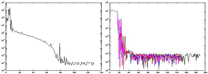 |
Figure 5: Typical shape of objective function derived from
CFD analysis.
![\begin{figure}\centering
\epsfig{figure=figures/noise3.eps,width=5cm, height=4...
...m]{
\epsfig{figure=figures/noise4b.eps,width=6cm,
height=4cm}}
\end{figure}](img899.png) |
A typical run for the optimization of the noisy Rosenbrock function is given in
the left of figure 4. Four typical runs for the optimization
of the simple noisy quadratic in four dimension are given in the right of figure
4. The noise on this four runs has an amplitude of
1e-4. In these conditions, CONDOR stops in average after 100 evaluations of the
objective function but we can see in figure 4 that
we usually already have found a quasi-optimum solution after only 45 evaluations.
As expected, there is a clear relationship between the noise applied on the objective
function and the average best value found by the optimizer. From the table 5.3
we can see the following: When you have a noise of  , the difference between the best value of the objective function
found by the optimizer AND the real value of the objective function at the optimum
is around
, the difference between the best value of the objective function
found by the optimizer AND the real value of the objective function at the optimum
is around  . In other words, in our case, if you apply a noise of
  , you will get a final value of the objective function around
. Obviously, this strange result only holds for this simple
objective function (the simple quadratic) and these particular testing conditions.
Nevertheless, the robustness against noise is impressive.
, you will get a final value of the objective function around
. Obviously, this strange result only holds for this simple
objective function (the simple quadratic) and these particular testing conditions.
Nevertheless, the robustness against noise is impressive.
If this result can be generalized, it will have a great impact in the field of
CFD shape optimization. This simply means that if you want a gain of magnitude
in the value of the objective function, you have to compute
your objective function with a precision of at least . This gives you an estimate of the precision at which you
have to calculate your objective function. Usually, the more precision, the longer
the evaluations are running. We are always tempted to lower the precision to gain
in time. If this strange result can be generalized, we will be able to adjust
tightly the precision and we will thus gain a precious time.
Given the search space comprised between 2 and 20 and given some noise of small
amplitude and high frequency on the objective function evaluation, among the best
optimizer available are UOBYQA and its parallel, constrained extension CONDOR.
When several CPU's are used, the experimental results tend to show that CONDOR
becomes the fastest optimizer in its category(fastest in terms of number of function
evaluations).
Some improvements are still possible:
- Add the possibility to start with a linear model, using a stable update
inspired by [36].
- Use a better strategy for the parallel case (see end of section 5.2)
- Currently the trust region is a simple ball (this is linked to the L2-norm
 used in step 4(a)ii of the algorithm). It would be
interesting to have a trust region which reflects the underlying geometry
of the model and not give undeserved weight to certain directions (for example,
using a H-norm) (see [9]). This improvement will have a small effect provided the
variables have already been correctly normalized.
used in step 4(a)ii of the algorithm). It would be
interesting to have a trust region which reflects the underlying geometry
of the model and not give undeserved weight to certain directions (for example,
using a H-norm) (see [9]). This improvement will have a small effect provided the
variables have already been correctly normalized.
Some research can also be made in the field of kriging models (see [4]). These models need very few "model improvement steps" to
obtain a good validity. The validity of the approximation can
also easily be checked.
The code of the optimizer is a complete C/C++ stand-alone package written
in pure structural programmation style. There is no call to fortran, external,
unavailable, copyrighted, expensive libraries. You can compile it under UNIX or
Windows. The only library needed is the standard TCP/IP network transmission library
based on sockets (only in the case of the parallel version of the code) which
is available on almost every platform. You don't have to install any special library
such as MPI or PVM to build the executables. The client on different platforms/OS'es
can be mixed together to deliver a huge computing power. The full description
of the algorithm code can be found in [39].
The code has been highly optimized (with extended use of memcpy function, special
fast matrix manipulation, fast pointer arithmetics, and so on...). However, BLAS
libraries [25] have not been used to allow a full Object-Oriented approach.
Anyway, the dimension of the problems is rather low so BLAS is nearly un-useful.
OO style programming allows a better comprehension of the code for the possible
reader.
A small C++ SIF-file reader has also been implemented (to be able to use the problems
coded in SIF from the CUTEr database, [33]). An AMPL interface [19] has also been implemented.
The fully stand-alone code is currently available at the homepage of the first
author: http://www.applied-mathematics.net.
-
- 1
- Aemdesign.
URL: http://www.aemdesign.com/FSQPapplref.htm.
- 2
- Paul T. Boggs and Jon W. Tolle.
Sequential Quadratic Programming.
Acta Numerica, pages 1-000, 1996.
- 3
- Andrew J. Booker, A.R. Conn, J.E. Dennis Jr., Paul D. Frank,
Michael Trosset, Virginia Torczon, and Michael W. Trosset.
Global modeling for optimization: Boeing/ibm/rice collaborative project 1995
final report.
Technical Report ISSTECH-95-032, Boeing Information Support Services, Research
and technology, Box 3707, M/S 7L-68, Seattle, Washington 98124, December 1995.
- 4
- Andrew J. Booker, J.E. Dennis Jr., Paul D. Frank, David B.
Serafini, Virginia Torczon, and Michael W. Trosset.
Optimization using surrogate objectives on a helicopter test example.
Computational Methods in Optimal Design and Control, pages 49-58,
1998.
- 5
- D. M. Bortz and C. T. Kelley.
The Simplex Gradient and Noisy Optimization Problems.
Technical Report CRSC-TR97-27, North Carolina State University, Department
of Mathematics, Center for Research in Scientific Computation Box 8205, Raleigh,
N. C. 27695-8205, September 1997.
- 6
- R. G. Carter, J. M. Gablonsky, A. Patrick, C. T. Kelley,
and O. J. Eslinger.
Algorithms for Noisy Problems in Gas Transmission Pipeline Optimization.
Optimization and Engineering, 2:139-157, 2001.
- 7
- Andrew R. Conn, Nicholas I.M. Gould, and Philippe L. Toint.
LANCELOT: a Fortran package for large-scale non-linear optimization (Release
A).
Springer Verlag, HeidelBerg, Berlin, New York, springer series in computational
mathematics edition, 1992.
- 8
- Andrew R. Conn, Nicholas I.M. Gould, and Philippe L. Toint.
Trust-region Methods.
SIAM Society for Industrial & Applied Mathematics, Englewood Cliffs, New
Jersey, mps-siam series on optimization edition, 2000.
Chapter 9: conditional model, pp. 307-323.
- 9
- Andrew R. Conn, Nicholas I.M. Gould, and Philippe L. Toint.
Trust-region Methods.
SIAM Society for Industrial & Applied Mathematics, Englewood Cliffs, New
Jersey, mps-siam series on optimization edition, 2000.
The ideal Trust Region: pp. 236-237.
- 10
- Andrew R. Conn, Nicholas I.M. Gould, and Philippe L. Toint.
Trust-region Methods.
SIAM Society for Industrial & Applied Mathematics, Englewood Cliffs, New
Jersey, mps-siam series on optimization edition, 2000.
Note on convex models, pp. 324-337.
- 11
- Andrew R. Conn, Nicholas I.M. Gould, and Philippe L. Toint.
A Derivative Free Optimization Algorithm in Practice.
Technical report, Department of Mathematics, University of Namur, Belgium,
98.
Report No. 98/11.
- 12
- Andrew R. Conn, K. Scheinberg, and Philippe L. Toint.
Recent progress in unconstrained nonlinear optimization without derivatives.
Mathematical Programming, 79:397-414, 1997.
- 13
- R. Cosentino, Z. Alsalihi, and R. Van Den Braembussche.
Expert System for Radial Impeller Optimisation.
In Fourth European Conference on Turbomachinery, ATI-CST-039/01,
Florence,Italy, 2001.
- 14
- Carl De Boor and A. A Ron.
On multivariate polynomial interpolation.
Constr. Approx., 6:287-302, 1990.
- 15
- J.E. Dennis Jr. and Robert B. Schnabel.
Numerical Methods for unconstrained Optimization and nonlinear Equations.
SIAM Society for Industrial & Applied Mathematics, Englewood Cliffs, New
Jersey, classics in applied mathematics, 16 edition, 1996.
- 16
- J.E. Dennis Jr. and V. Torczon.
Direct search methods on parallel machines.
SIAM J. Optimization, 1(4):448-474, 1991.
- 17
- J.E. Dennis Jr. and H.F. Welaker.
Inaccurracy in quasi-Newton methods: local improvement theroems.
Mathematical programming Study, 22:70-85, 1984.
- 18
- R. Fletcher.
Practical Methods of optimization.
a Wiley-Interscience publication, Great Britain, 1987.
- 19
- Robert Fourer, David M. Gay, and Brian W. Kernighan.
AMPL: A Modeling Language for Mathematical Programming.
Duxbury Press / Brooks/Cole Publishing Company, 2002.
- 20
- P.E. Gill, W. Murray, M.A. Saunders, and Wright M.H.
Users's guide for npsol (version 4.0): A fortran package for non-linear programming.
Technical report, Department of Operations Research, Stanford University,
Stanford, CA94305, USA, 1986.
Report SOL 862.
- 21
- P. Gilmore and C. T. Kelley.
An implicit filtering algorithm for optimization of functions with many local
minima.
SIAM Journal of Optimization, 5:269-285, 1995.
- 22
- Nicholas I. M. Gould, Dominique Orban, and Philippe L. Toint.
CUTEr (and SifDec ), a Constrained and Unconstrained Testing Environment,
revisited .
.
Technical report, Cerfacs, 2001.
Report No. TR/PA/01/04.
- 23
- W. Hock and K. Schittkowski.
Test Examples for Nonlinear Programming Codes.
Lecture Notes en Economics and Mathematical Systems, 187, 1981.
- 24
- C. T. Kelley.
Iterative Methods for Optimization, volume 18 of Frontiers
in Applied Mathematics.
Philadelphia, 1999.
- 25
- C. L. Lawson, R. J. Hanson, D. Kincaid, and F. T. Krogh.
Basic Linear Algebra Subprograms for FORTRAN usage.
ACM Trans. Math. Soft., 5:308-323, 1979.
- 26
- J.J. Moré and D.C. Sorensen.
Computing a trust region step.
SIAM journal on scientif and statistical Computing, 4(3):553-572,
1983.
- 27
- Eliane R. Panier and André L. Tits.
On combining feasibility, Descent and Superlinear Convergence in Inequality
Contrained Optimization.
Mathematical Programming, 59:261-276, 1995.
- 28
- S. Pazzi, F. Martelli, V. Michelassi, Frank Vanden Berghen,
and Hugues Bersini.
Intelligent Performance CFD Optimisation of a Centrifugal Impeller.
In Fifth European Conference on Turbomachinery, Prague, CZ, March
2003.
- 29
- Stéphane Pierret and René Van den Braembussche.
Turbomachinery blade design using a Navier-Stokes solver and artificial neural
network.
Journal of Turbomachinery, ASME 98-GT-4, 1998.
publication in the transactions of the ASME: '' Journal of Turbomachinery
''.
- 30
- C. Poloni.
Multi Objective Optimisation Examples: Design of a Laminar Airfoil and of
a Composite Rectangular Wing.
Genetic Algorithms for Optimisation in Aeronautics and Turbomachinery,
2000.
von Karman Institute for Fluid Dynamics.
- 31
- M.J.D. Powell.
A direct search optimization method that models the objective and constraint
functions by linar interpolation.
In Advances in Optimization and Numerical Analysis, Proceedings of the
sixth Workshop on Optimization and Numerical Analysis, Oaxaca, Mexico,
volume 275, pages 51-67, Dordrecht, NL, 1994. Kluwer Academic Publishers.
- 32
- M.J.D. Powell.
The use of band matrices for second derivative approximations in trust region
algorithms.
Technical report, Department of Applied Mathematics and Theoretical Physics,
University of Cambridge, England, 1997.
Report No. DAMTP1997/NA12.
- 33
- M.J.D. Powell.
On the Lagrange function of quadratic models that are defined by interpolation.
Technical report, Department of Applied Mathematics and Theoretical Physics,
University of Cambridge, England, 2000.
Report No. DAMTP2000/10.
- 34
- M.J.D. Powell.
UOBYQA: Unconstrained Optimization By Quadratic Approximation.
Technical report, Department of Applied Mathematics and Theoretical Physics,
University of Cambridge, England, 2000.
Report No. DAMTP2000/14.
- 35
- M.J.D. Powell.
UOBYQA: Unconstrained Optimization By Quadratic Approximation.
Mathematical Programming, B92:555-582, 2002.
- 36
- M.J.D. Powell.
On updating the inverse of a KKT matrix.
Technical report, Department of Applied Mathematics and Theoretical Physics,
University of Cambridge, England, 2004.
Report No. DAMTP2004/01.
- 37
- Thomas Sauer and Yuan Xu.
On multivariate lagrange interpolation.
Math. Comp., 64:1147-1170, 1995.
- 38
- D. E. Stoneking, G. L. Bilbro, R. J. Trew, P. Gilmore,
and C. T. Kelley.
Yield optimization Using a gaAs Process Simulator Coupled to a Physical Device
Model.
IEEE Transactions on Microwave Theory and Techniques, 40:1353-1363,
1992.
- 39
- Frank Vanden Berghen.
Intermediate Report on the development of an optimization code for smooth,
continuous objective functions when derivatives are not available.
Technical report, IRIDIA, Université Libre de Bruxelles, Belgium, 2003.
Available at http://www.applied-mathematics.net/optimization/.
- 40
- Frank Vanden Berghen.
Optimization algorithm for Non-Linear, Constrained, Derivative-free optimization
of Continuous, High-computing-load Functions.
Technical report, IRIDIA, Université Libre de Bruxelles, Belgium, 2004.
Available at http://iridia.ulb.ac.be/ fvandenb/work/thesis/.
- 41
- J. F. Wanga, J. Periaux, and Sefriouib M.
Parallel evolutionary algorithms for optimization problems in aerospace engineering.
Journal of Computational and Applied Mathematics, 149, issue 1:155-169,
December 2002.
- 42
- D. Winfield.
Function and functional optimization by interpolation in data tables.
PhD thesis, Harvard University, Cambridge, USA, 1969.
- 43
- D. Winfield.
Function minimization by interpolation in a data table.
Journal of the Institute of Mathematics and its Applications, 12:339-347,
1973.
Frank Vanden Berghen 2004-08-16