LARS Library: Least Angle Regression laSso Library
Frank Vanden Berghen
The PDF version of this page is available here.
You can download here the
LARS library ( v1.06 - released 2/10/2007) (new binaries that works on any windows-matlab
version).
Let's assume that we want to perform a simple identification task. Let's assume
that you have a set of  measures
 . We want to find a function (or
a model) that predicts the measure
. We want to find a function (or
a model) that predicts the measure  in function of the measures
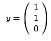
 . The vector
 has several names:
 is the regressor vector.
 - is the input.
- is the vector of independent variables.
has several names:
- is the target.
- is the output.
- ( is the dependant variable).
The pair  has several names:
- is an input
 output pair.
- is a sample.
We want to find  such that
  . Let's also assume that you know that
  belongs to the family of linear models. I.e.
 where
where
 is the dot product of two vectors and
  is the constant term. You can also write
 where
where
 and are describing . We will now assume, without loss of generality, that
  . We will see later how to compte if this is not the case.
  is the model that we want to find. Let's now assume
that we have many input
output pairs. i.e. we have
is the model that we want to find. Let's now assume
that we have many input
output pairs. i.e. we have
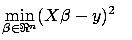
We want to compute such that
 . Using matrix notation, is the solution of:
 |
(2) |
where
 is a matrix containing on each line a different
regressor and
is a matrix containing on each line a different
regressor and
 contains all the targets. The columns of
  contain the independent variables or, in short, the variables.
If
contain the independent variables or, in short, the variables.
If  , we can compute using a simple Gauss-Jordan elimination. That's not very interesting.
We are usually more interested in the case where
, we can compute using a simple Gauss-Jordan elimination. That's not very interesting.
We are usually more interested in the case where  : when the linear system
  is over-determined. We want to find
  such that the Total Prediction Error (TPError) is
minimum:
such that the Total Prediction Error (TPError) is
minimum:
TPError |
(3) |
If we define the total prediction error
TPError as
Sum of Squared Errors
where
 is the
  -norm of a vector, we obtain the Classical Linear Regression
or Least Min-Square(LS):
-norm of a vector, we obtain the Classical Linear Regression
or Least Min-Square(LS):
Classical Linear Regression: is the solution to:
Such a definition of the total prediction error
TPError can give un-deserved weight to a small number of bad samples.
It means that one sample with a large prediction error is enough to change
completely (this is due to the squaring effect that ``amplifies'' the
contribution of the ``outliers''). This is why some researcher use a  instead of a
  :
:
Robust Regression: is the solution to:
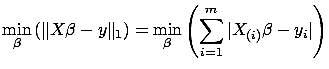
where  is the absolute value. We will not discuss here
Robust regression algorithms. To find the solution of a classical Linear
Regression, we have to solve:
is the absolute value. We will not discuss here
Robust regression algorithms. To find the solution of a classical Linear
Regression, we have to solve:
Since
 is a scalar, we can take its transpose without changing
its value:
is a scalar, we can take its transpose without changing
its value:
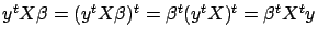 . We obtain:
The equation 4 is the well-known normal equation.
On the left-hand-side of this equation we find
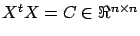 : the correlation matrix.
  is symmetric and semi-positive definite (all the eigenvalues of are
  ). The element
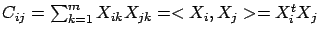 is the correlation between column
  and column
  (where
  stands for column of ). The right-hand-side of equation 4 is also
interesting: it contains the univariate relation of all the columns of (the variables) with the target .
stands for column of ). The right-hand-side of equation 4 is also
interesting: it contains the univariate relation of all the columns of (the variables) with the target .
We did previously the assumption that the constant term of the model is zero. is null when  and
and
 where
where
 is the mean operator and is the
  column of . Thus, in the general case, when
  , the procedure to build a model is:
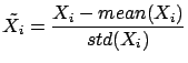
- Compute
 where
where
 is the ``standard deviation'' operator.
- Normalize the target:
- Normalize the columns of :
- Since the columns of
 have zero mean, and since
  has zero mean, we have . We can thus use the normal equations:
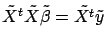 to find
 . All the columns inside have a standard deviation of one. This increase numerical
stability.
. All the columns inside have a standard deviation of one. This increase numerical
stability.
- Currently,
has been computed on the ``normalized columns''
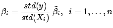
 and . Let's convert back the model so that it can be applied on the
un-normalized and :
and . Let's convert back the model so that it can be applied on the
un-normalized and :
From now on, in the rest of this paper, we will always assume that (data has been normalized).
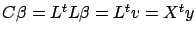
One simple way to solve the normal equations 4
is the following:
- Compute a Cholesky factorization
 of
of  . i.e. Compute such that is a lower triangular matrix and such that
  .
.
- Let's define
 . Then we have:
 (the last equality comes from equation 4).
This last equation (
(the last equality comes from equation 4).
This last equation (
 )can be solved easily because
  is triangular. Once we have found
  , we solve
 to find (this is also easy because is triangular).
Unfortunately, the above algorithm is not always working properly. Let's consider
the case where  . i.e. the variables and are 100% linearly correlated together. In this case, we will have
 .
.  can be any value at the condition that
 (so that we obtain
 and none of the columns and are meaningful to predict ). Thus, can become extremely large and give undeserved weight to the
column . We have one degree of liberty on the 's. This difficulty arises when:
and none of the columns and are meaningful to predict ). Thus, can become extremely large and give undeserved weight to the
column . We have one degree of liberty on the 's. This difficulty arises when:
- A column of is a linear combination of other columns.
- The rank of A is lower than
 .
.
- The matrix is not of full rank .
This problem is named the ``multi-colinearity problem''. It is illustrated in
figure 1 and 2.
Figure 1: Stable Model
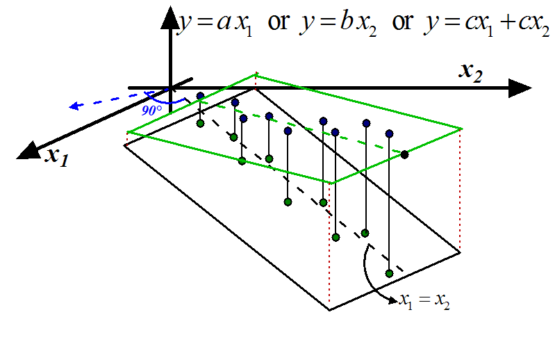 |
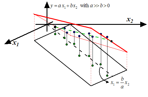
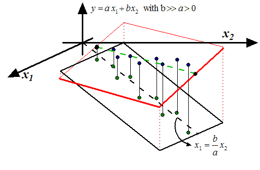
Figure 2: Unstable Models
  |
The blue points inside figures 1 and 2
are the samples. The green points are the lines of
 (the inputs) and the heights of the
blue points are the targets (
(the inputs) and the heights of the
blue points are the targets (
 )(the output). There is a linear correlation between
 and
and  :
:
 . In the ``blue direction'' (perpendicular to
the black dashed line), we do not have enough reliable information to decide if
the output should increase or decrease. Inside figures 1
and 2, a model is represented by a plane. In this situation, the ideal model
that we want to obtain, is drawn in green in figure 1
(the plane/model is ''flat'': there is no un-due variation of in the ``blue direction''). The equation of the ideal model is either:
. In the ``blue direction'' (perpendicular to
the black dashed line), we do not have enough reliable information to decide if
the output should increase or decrease. Inside figures 1
and 2, a model is represented by a plane. In this situation, the ideal model
that we want to obtain, is drawn in green in figure 1
(the plane/model is ''flat'': there is no un-due variation of in the ``blue direction''). The equation of the ideal model is either:
 or
or  or
or
 . Note that, inside figure 2
(and also 1), we do NOT have exactly
. Note that, inside figure 2
(and also 1), we do NOT have exactly
 (the green point are not totally on the dashed line
 ). Thus, we theoretically have enough information
in the ``blue direction'' to construct a model. However exploiting this information
to predict is not a good idea and leads to unstable models: a small perturbation
of the data ( or ) leads to a completely different model: Inside figure 2,
we have represented in red two models based on small perturbations of and . Usually, unstable models have poor accuracy. The main question now
is: How to stabilize a model? Here are two classical solutions:
). Thus, we theoretically have enough information
in the ``blue direction'' to construct a model. However exploiting this information
to predict is not a good idea and leads to unstable models: a small perturbation
of the data ( or ) leads to a completely different model: Inside figure 2,
we have represented in red two models based on small perturbations of and . Usually, unstable models have poor accuracy. The main question now
is: How to stabilize a model? Here are two classical solutions:
- Inside figure 1, the 'information' that is
contained in is duplicated in . We can simply drop one of the two variables. We obtain the models
or . The main difficulty here is to select carefully the columns
that must be dropped. The solution is the ``LARS/Lasso Algorithm'' described
later in this paper.
- The other choice is to keep inside the model
 all the variables (
 and
and
 ). However, in this case, we must be sure that:
-

 and
and  are small values (I remind you that and can become arbitrarily large).
We must find an algorithm to compute that will ``equilibrate'' and ``reduce'' the 's:

is the solution of
 |
(5) |
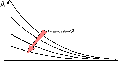
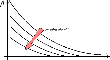
This technique is named ``Ridge regression''. When

increases, all the
are ``equilibrated'' and ``pushed'' to zero as illustrated
in figure
3.
Figure 3: The 's sorted from greatest to smallest for different value of
.
 |
We will discuss later of a way to compute an optimal regularization parameter
. Inside figure
1, we obtain
the model
and we have thus
with

''small''.
The ``Ridge regression'' technique is particularly simple and efficient. It has
a nice graphical explanation. The ``Ridge
regression'' technique is in fact searching for that minimizes
 Squared Error
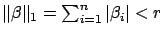
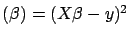 under the constraint that
 . This definition is illustrated on the left
of figure 4.
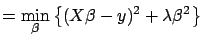
We seek the solution of the minimization problem:
. This definition is illustrated on the left
of figure 4.
We seek the solution of the minimization problem:
subject to

(with  and
and  ) To solve this minimization problem, we first have to rewrite
the constraint:
) To solve this minimization problem, we first have to rewrite
the constraint:
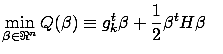
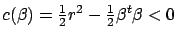 . Now, we introduce
a Lagrange multiplier and the Lagrange function:
Using the Lagrange First order optimality criterion, we know that the solution
. Now, we introduce
a Lagrange multiplier and the Lagrange function:
Using the Lagrange First order optimality criterion, we know that the solution
 to this optimization problem is given by:
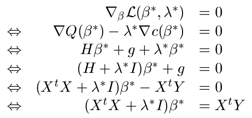 |
(6) |
which is equation 5.
Figure 4: On the left: Illustration of Ridge Regression.
On the right: Illustration of Lasso
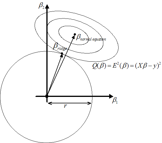 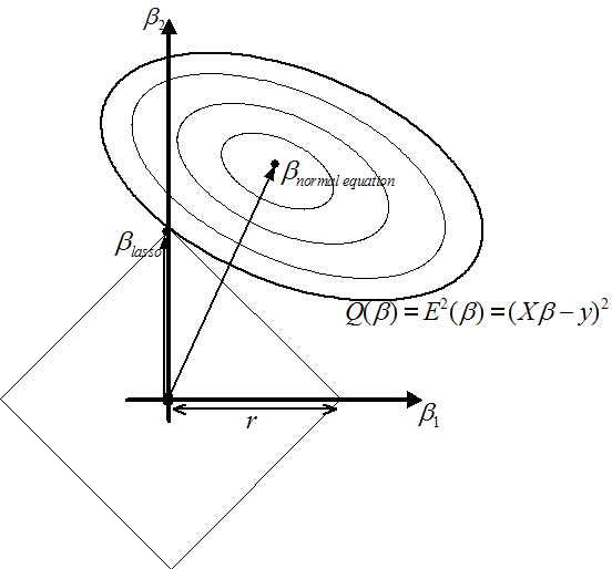 |
The constraint
prevents the 's from becoming arbitrarily large. As illustrated in figure
3, the ridge regression algorithm ``pushes'' all the
's towards zero but none of the actually gets a null value. It's interesting to have  because, in this case, we can completely remove from the
model the column . A model that is using less variables has many advantages: it is
easier to interpret for a human and it's also more stable. What happens if we
replace the constraint
with the constraint
because, in this case, we can completely remove from the
model the column . A model that is using less variables has many advantages: it is
easier to interpret for a human and it's also more stable. What happens if we
replace the constraint
with the constraint
 ? See the
right of illustration 4. You can see on the figure that
? See the
right of illustration 4. You can see on the figure that
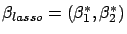 with
with
 . You can see on figure 5 that,
as you decrease
. You can see on figure 5 that,
as you decrease  , more and more
  are going to zero.
Figure 5: The 's sorted from greatest to smallest for different values of
|
The Lasso regression is defined by: is the solution of the minimization problem:
 subject to subject to  |
(7) |
As you can see, computing different 's (with a different number of null 's) involves solving several times equation 7
for different values of . Equation 7 is a QP (Quadratic Programming)
problem and is not trivial to solve at all. The Lasso algorithm, as it is described
here, is thus very demanding on computer resources and is nearly of no practical
interest. Hopefully, there exist another, more indirect, way to compute at a very
little cost all the solutions of the Lasso Algorithm for all the values of . A modification of the LARS algorithm computes all the Lasso solution
in approximatively the time needed to compute and solve the simple ``normal equations''
(equation 4) (the algorithmic complexity of
the two procedures is the same). LARS stands for ``Least Angle Regression laSso''.
We will not describe here the LARS algorithm but we will give an overview of some
of its nicest properties.
The LARS algorithm is a refinement of the FOS (Fast Orthogonal Search) algorithm.
We will start by describing the FOS algorithm. The FOS (and the LARS algorithm)
is a forward stepwise algorithm. i.e. FOS is an iterative algorithm that, at each
iteration, includes inside its model a new variable. The set of variables inside
the model at iteration  is the ``active set''

 . The set of variables outside the model is the ``inactive set''
 .
.
 is a subset of column of containing only the active variables at iteration .
 is a subset of column of containing only the inactive variables at iteration .
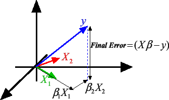
Let's first illustrate the equation 2: . Equation 2 can be rewritten:
 |
(8) |
If
, then
 is a column of X. can also be seen as a vector in a
  dimensional space and
is the best linear combination of the vectors to reach the target . The ``vector view'' of equation 8 is illustrated
in figure 6 where
dimensional space and
is the best linear combination of the vectors to reach the target . The ``vector view'' of equation 8 is illustrated
in figure 6 where
Figure 6: Graphical interpretation of
|
The FOS algorithm does the following:
- Let's define the residual prediction error at step as
 . We have
  . Normalize the variables and the target to have
 and
and  . Set
. Set  , the iteration counter.
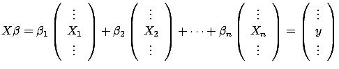
Figure 7: Illustration of the FOS algorithm
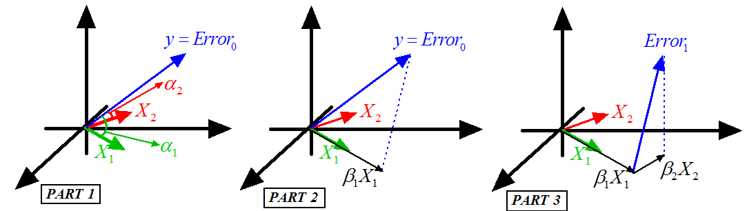 |
- This step is illustrated in figure 7, Part 1.
We will add inside
the variable that is ``the most in the direction of ''. i.e. the ``angle''
 between
  and is smaller than all the other angles
  (
( ) between the 's and . Using the well-know relation:
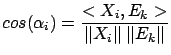 |
(9) |
Since the variables have been normalized, we obtain:
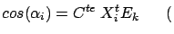 where where  |
(10) |
Note that  is simply the correlation between variable and the Residual Error .
Thus the algorithm is: ``compute
 . Find such that
 |
(11) |
Add the variable to the active set
. Remove variable from the inactive set
''.
- This step is illustrated in figure 7, Part 2.
We now compute
 , the length of the ``step'' in the direction (inside the example j=1). Let's project (orthogonally)
inside the space that is ``spanned'' by the active variables. The
projection of is named
, the length of the ``step'' in the direction (inside the example j=1). Let's project (orthogonally)
inside the space that is ``spanned'' by the active variables. The
projection of is named  . We obtain
 since is normalized. If the projection operator fails ( is
inside the space spanned by the active set  of variables), remove from the active set
and go to step 2.
of variables), remove from the active set
and go to step 2.
- Deflation: update of the Residual Error:
 .
.
- If
is empty then stop, otherwise increment and go to step 2.
Let's define  , the number of active variable at the end of the algorithm. If
you decide to stop prematurely (for example, when
, the number of active variable at the end of the algorithm. If
you decide to stop prematurely (for example, when
 ), you will have
  . The FOS algorithm has several advantages:
- It's ultra fast! Furthermore, the computation time is mainly proportional
to . If , then you will go a lot faster than when using the standard
normal equations.
- The algorithm will ``avoid'' naturally the correlated columns. I remind
you that a model that is using two strongly correlated columns is likely to
be unstable. If column and are strongly correlated, they are both ``pointing'' to the same direction
(the angle between them is small: see equation 9
and figure 6) . If you include inside the active
set the column , you will obtain, after the deflation, a new error
 that will prevent you to choose at a later iteration. One interpretation is the following: ``All
the information contained inside the direction has been used. We are now searching for other directions to reach
''. It is possible that, at the very end of the procedure, the algorithm
still tries to use column . In this case, the projection operator used at step 3 will fail
and the variable will be definitively dropped. Models produced with the FOS algorithm
will thus be usually very stable.
that will prevent you to choose at a later iteration. One interpretation is the following: ``All
the information contained inside the direction has been used. We are now searching for other directions to reach
''. It is possible that, at the very end of the procedure, the algorithm
still tries to use column . In this case, the projection operator used at step 3 will fail
and the variable will be definitively dropped. Models produced with the FOS algorithm
will thus be usually very stable.
- The selection of the column that enters the active set is based on the ``residual
error'' at step (with
 ). This selection is thus exploiting the information contained
inside the target . The ``target information'' is not used by other algorithms that
are based on SVD of or QR factorization of . The FOS algorithm will thus performs a better variable selection
than SVD- or QR-based algorithm. Many other algorithms do not use any deflation.
Deflation is important because it allows us to search for variables that explains
the part of the target that is still un-explained (the residual error ). A good variable selection is useful when .
). This selection is thus exploiting the information contained
inside the target . The ``target information'' is not used by other algorithms that
are based on SVD of or QR factorization of . The FOS algorithm will thus performs a better variable selection
than SVD- or QR-based algorithm. Many other algorithms do not use any deflation.
Deflation is important because it allows us to search for variables that explains
the part of the target that is still un-explained (the residual error ). A good variable selection is useful when .
- The memory consumption is very small. To be able to use the FOS algorithm,
you only need to be able to store in memory the target , one line of , and a dense triangular matrix of dimension Other algorithms based on QR factorization of requires to have the full matrix inside memory because the memory space used to store is used during the QR factorization to store temporary, intermediate
results needed for the factorization. Algorithms based on SVD of are even more memory hungry. This is a major drawback for most advanced
applications, especially in Econometrics where we often have
 . There exists some ``out of core'' QR and SVD factorizations that
are able to work even when does not fit into memory. However ``out of core'' algorithms are
currently extremely slow and unstable.
. There exists some ``out of core'' QR and SVD factorizations that
are able to work even when does not fit into memory. However ``out of core'' algorithms are
currently extremely slow and unstable.
There is however one major drawback to the FOS algorithm. It is illustrated in
figure 8 where we have:
Figure: FOS algorithm fails and gives
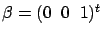
 |
At the first iteration, the FOS algorithm selects  because
 is greater than
 (and
(and  . Thereafter, the FOS algorithm computes the new Residual Error
 and get stuck. Indeed, if we add to the active
set either or , the L2-norm of the Residual Error do not decrease:
and get stuck. Indeed, if we add to the active
set either or , the L2-norm of the Residual Error do not decrease:
 . There is no way to add a new variable
to decrease the Residual Error and thus the algorithm stops. There are mainly
two conceptual reasons why the FOS algorithm fails:
. There is no way to add a new variable
to decrease the Residual Error and thus the algorithm stops. There are mainly
two conceptual reasons why the FOS algorithm fails:
- The FOS algorithm is a forward stepwise algorithm and, as almost all forward
stepwise algorithms, it is not able to detect multivariate concepts. In the
example illustrated in figure 8, the target is defined
precisely to be =+. You are able to predict the target accurately if your model is
 . The FOS algorithm gives the wrong model
. In this example, the target is a multivariate concept hidden inside two variables: and . A forward stepwise algorithm that is able to detect a multivariate
concept is very difficult to develop. Inside FOS, the selection of the variable
that enters the active set is only based on the univariate relation
of with the target . On the contrary, Backward stepwise algorithms have no problem to
detect multi-variable concepts and should thus be preferred to a Simple,Classical
Forward Stepwise Algorithm. However, usually, Backward stepwise algorithms
are very time consuming because they need first to compute a full model and
thereafter to select carefully which variables they will drop.
. The FOS algorithm gives the wrong model
. In this example, the target is a multivariate concept hidden inside two variables: and . A forward stepwise algorithm that is able to detect a multivariate
concept is very difficult to develop. Inside FOS, the selection of the variable
that enters the active set is only based on the univariate relation
of with the target . On the contrary, Backward stepwise algorithms have no problem to
detect multi-variable concepts and should thus be preferred to a Simple,Classical
Forward Stepwise Algorithm. However, usually, Backward stepwise algorithms
are very time consuming because they need first to compute a full model and
thereafter to select carefully which variables they will drop.
The LARS algorithm with Lasso modification is a forward stepwise algorithm
that produces all the solutions of the Lasso algorithm in a computing time
proportional to ( is the number of active variable at the end of the algorithm).
The Lasso algorithm is part of the family of the backward stepwise algorithm
(It starts with a full model and remove some variables when decreases). Thus, the Lasso algorithm is able to discover multi-variable
concepts. And thus, the LARS algorithm with Lasso modification is also able
to discover multi-variable concepts (since LARS with Lasso gives the same
models than the Lasso algorithm). From my knowledge, the LARS algorithm with
Lasso modification is the only forward stepwise algorithm able to discover
multi-variable concepts. Since, it's a forward stepwise algorithm, it's also
very fast.
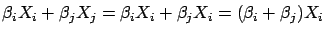
On the other side, conjunctive concepts are easy to detect. Let's assume that
you have the following:
If you create a column
 (
(
 ), you obtain:
and
i.e. You can represent conjunctive concepts with the product of variables.
You will thus obtain second order models. Computing second order models usually
involves extending the original matrix with columns that are the product of some of the columns of
the original . This is usually a very memory expansive operation. Indeed if is the number of column of , then the extended
 matrix has
 columns. The LARS library has been built to allow
you to easily create ``on the fly'' a regressor (= one line of
). i.e. you only need to be able to store in memory one
line of
, not the whole
matrix. This allows you to compute at a low memory consumption
second, third, fourth,... order models.
columns. The LARS library has been built to allow
you to easily create ``on the fly'' a regressor (= one line of
). i.e. you only need to be able to store in memory one
line of
, not the whole
matrix. This allows you to compute at a low memory consumption
second, third, fourth,... order models.
- The FOS algorithm is ``too greedy'': when the FOS algorithm finds a good
direction, it is exploiting this direction ``to the maximum'' (the length
of the steps is
 ). Thereafter there is no ``room left'' for further
improvements, adding other variables. The FOS has been ``trapped'' in a so-called
``local optimum''. The LARS algorithm is not so greedy. Its steps lengthes
are shorter (see step 3. of the FOS algorithm about ``steps''). This means
that the different models that are computed at each steps of the LARS algorithm
are not 100% efficient. With the same set of active variables, one can compute
a better model. The LARS library downloadable on this page allows you to obtain
both models:
). Thereafter there is no ``room left'' for further
improvements, adding other variables. The FOS has been ``trapped'' in a so-called
``local optimum''. The LARS algorithm is not so greedy. Its steps lengthes
are shorter (see step 3. of the FOS algorithm about ``steps''). This means
that the different models that are computed at each steps of the LARS algorithm
are not 100% efficient. With the same set of active variables, one can compute
a better model. The LARS library downloadable on this page allows you to obtain
both models:
- the most efficient one.
- the one used inside the LARS algorithm to search for the next variables
to add inside the active set.
To resume, the LARS algorithm has all the advantages of the FOS algorithm:
- ultra fast.
- correlated columns are avoided to obtain stable models.
- Selection of the active variables based on the target (Deflation).
- small memory consumption.
Furthermore, the LARS algorithm with Lasso modification is able to discover multivariate
concepts easily. For example, the LARS algorithm with LASSO modification finds
for the example illustrated in figure 8 .
There exists one last question to answer when using the LARS algorithm: When to
stop? How to choose ? The question is not simple. Several strategies are available inside
the LARS library downloadable on this page:
My advice is :
- to choose a very stringent termination test (like the first one with
 ) to be sure to have all the informative variables.
  has a nice and easy interpretation: it's the percentage of
the variance inside that will not be explained.
- to perform a backward stepwise, using as initial model, the model given
by the LARS algorithm. The LARS library has been designed so that such task
is very easy to code.
My experience is that stopping criterions based on MDL (maximum description
length), Akkaike index or  statistics are not reliable.
To be able to answer the simple question ``How good is my model?'' you need a
good methodology. Let's assume that we have a set of data and . You will cut this data in three parts: a creation set  , a validation set
  and a test set
  . The procedure is illustrated in figure 9.
Figure 9: Data are cut into three parts
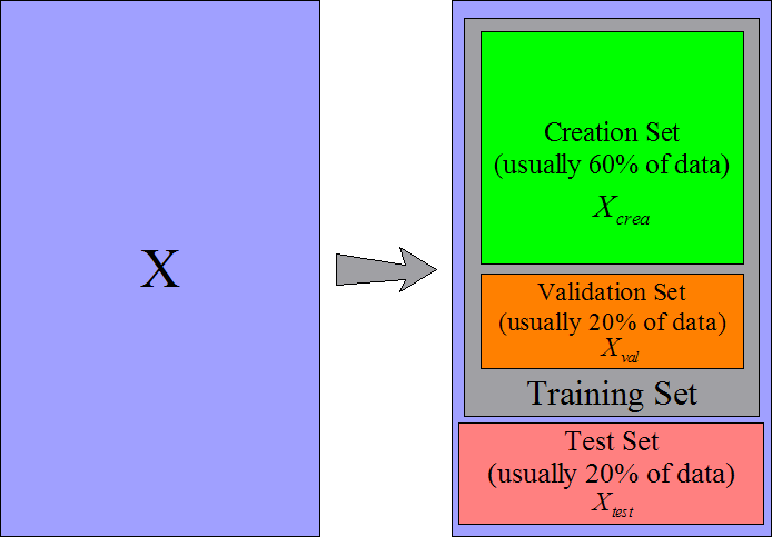 |
The creation set will be used to build a first model. You can build the model
using the normal equation (
 ) or using the LARS algorithm. Thereafter
the model needs to be stabilized (stabilization is less important if you
have built the model with the LARS algorithm but can still improve a little your
model). There are mainly two simple ways to stabilize a model: Remove un-informative
variables (this is called ''backward stepwise'') and Ridge Regression.
) or using the LARS algorithm. Thereafter
the model needs to be stabilized (stabilization is less important if you
have built the model with the LARS algorithm but can still improve a little your
model). There are mainly two simple ways to stabilize a model: Remove un-informative
variables (this is called ''backward stepwise'') and Ridge Regression.
To remind you, the Ridge Regression is based on equation 5:
 |
(17) |
where is the regularization parameter that needs to be adjusted,
 is the model (depending on the value of ) and is the creation set. If is high, the model will be strongly stabilized. The optimal
value of the parameter is
is the model (depending on the value of ) and is the creation set. If is high, the model will be strongly stabilized. The optimal
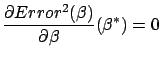
value of the parameter is  . is the solution to the optimization problem:
where
is computed from equation 17.
We are searching for the value of that gives the best model when applied on the validation set.
We are improving the ``generalization ability'' of our model. Since we never used
any data from the validation set to build our model, the performance of the model
is entirely due to its ``generalization ability''.
. is the solution to the optimization problem:
where
is computed from equation 17.
We are searching for the value of that gives the best model when applied on the validation set.
We are improving the ``generalization ability'' of our model. Since we never used
any data from the validation set to build our model, the performance of the model
is entirely due to its ``generalization ability''.
To stabilize your model, you can also completely remove some variables using a
``backward stepwise'' algorithm. Here is a simple ``backward stepwise'' algorithm:
- Let's define
 , the creation set without the column . Let's define
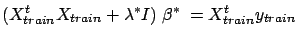
 where is the solution to the standard normal equation:
 .
.  is the performance on the validation set of a model using all the columns of the creation set . Set
  .
.
- We will try to remove the variable . Compute
 , the solution to
 . Compute
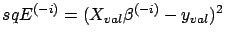 : the performance of
the model
on the validation set when the model is built without taking into account the column of the creation set . If
: the performance of
the model
on the validation set when the model is built without taking into account the column of the creation set . If
 , then the column did not contain any information and can be dropped: Set
 .
.
- Choose another and go back to step 2.
Let's define
, the optimal set of column after the backward stepwise.
Once we have found an optimal ridge parameter and/or the optimal set
of informative columns (backward stepwise), we can
compute the final model using:
 |
(18) |
where  contains only the columns in
.
contains only the columns in
.
WARNING: If you try to use both regularization techniques at the same time, they
will ``enter in competition''. You should then be very careful.
To get an idea of the quality of your final model , you can apply it on the test set:
Squared Error on test set=
The methodology just described here is a correct approach to a modelization problem.
However, this approach does not use a very large validation and test set. Since
the validation set is small, the parameter and the set
of active columns will be very approximative. Since
the test set is small, the estimation of the quality of the model is also very
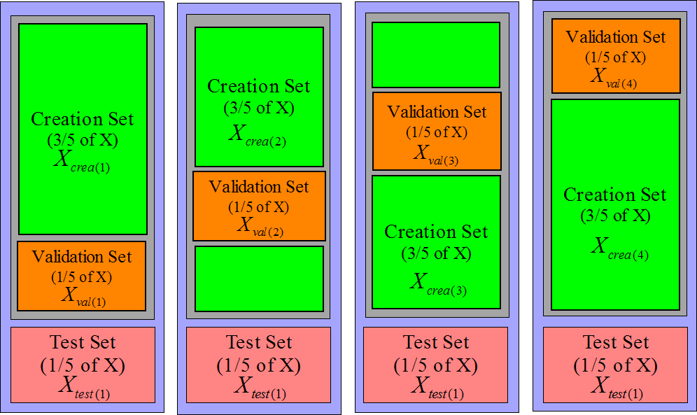
approximative. To overcome these difficulties, we can use a n-fold-cross-validation
technique. If we want a more accurate estimation of the quality of the model,
we can build 5 test sets instead of one: see figure 10.
It's named a 5-fold-cross-validation. It also means that we have 5 training sets
and thus 5 different models. The main point here is that none of these 5 models
have seen the data that are inside their corresponding test set.
Figure 10: 5 test sets (and 5 training sets))
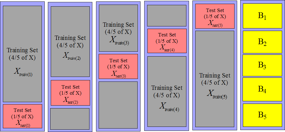 |
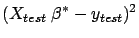
An estimation of the overall quality of our modelization is:
| |
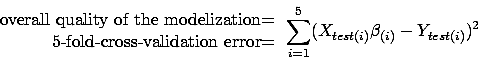 |
|
| |
where
 is the solution to is the solution to 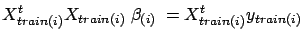 |
(19) |
where
 and
and
 are defined on figure 10.
When we perform a n-fold-cross-validation, we must compute different models
 using equation 19.
The only time-consuming part inside equation 19 is
the computation of
using equation 19.
The only time-consuming part inside equation 19 is
the computation of
 . Here is a small ``trick'' to be able to compute
 in a very efficient way:
If we define
in a very efficient way:
If we define  as in figure 10, we can compute
 . Then, we have:
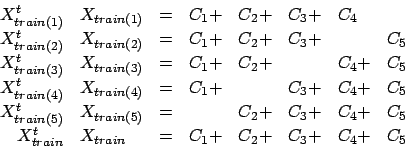 |
(20) |
Thanks to equations 20, we can compute
very easily: only a few matrix
additions are needed. The same property of addition exist for the right hand side
of equation 19:
 . Since solving equation 19 is instantaneous
on modern CPU's (only the computation of
. Since solving equation 19 is instantaneous
on modern CPU's (only the computation of
 is time-consuming), we can easily obtain the
 different models
and the n-fold-cross-validation is ``given nearly for free''.
different models
and the n-fold-cross-validation is ``given nearly for free''.
The same technique can be applied to increase the size of the validation set:
see figure 11.
Figure 11: 4 validation sets (and 4 creation sets))
 |
When building a model, the first step is the normalization of all the variables
(the columns ). The normalization of a variable consist of two steps:
- We subtract from the column its mean

- We divide the column by its standard deviation

Thereafter the
 are computed: see equation 20 and
figure 10. Based on the
are computed: see equation 20 and
figure 10. Based on the  's we can compute easily many different models
. Let's assume that we want a model that is completely ignoring
the block
's we can compute easily many different models
. Let's assume that we want a model that is completely ignoring
the block  : the block will be used as test set. Referring to figure 10,
the test set is
: the block will be used as test set. Referring to figure 10,
the test set is
 and the training set is
 . The columns in block
  have been normalized using and . The two parameters and are partially based on information contained inside the block
. We are breaking the rule that says:
have been normalized using and . The two parameters and are partially based on information contained inside the block
. We are breaking the rule that says:
| ``never use any information from the test set
to build a model'' |
(21) |
The columns in (part of the creation set) are normalized using information from
(the test set). This small ``infraction'' of the rules is usually
negligible and allows us to reduce considerably the computation time. However,
for some rare variables, the rule must be respected strictly. These variables
are named ``dynamic variables''. The LARS library does a strong distinction between
``dynamic variables'' and ``static variables''. The LARS library handles both
types of variables. However only the ''static variables'' are reviewed inside
this documentation.
The concept of ``dynamic variables'' is linked with the concept of ``variable
recoding''. The normalization of the variables is a (very basic) recoding. If
there is no recoding, there is no ``dynamic variables''. The ``normalization of
a variable'' is a recoding that never produces any ``dynamic variables'' (especially
if all the lines of have been correctly scrambled). ``Dynamic variables'' appears mostly
when using advanced recodings such as, for example, in the paper ``1-Dimensional
Splines as Building Blocks for Improving Accuracy of Risk Outcomes Models'' by
David S. Vogel and Morgan C. Wang. The LARS library is handling advanced recodings
through the use of ``dynamic variables''.
Inside the LARS library, the parameter of the Ridge Regression is computed using a n-fold-cross-validation
on the validation sets. Equations 20 are used to achieve
high efficiency. The
 matrices are built incrementally each
time a new variable enters the active set
. The equations 19 are solved
using an advanced Cholesky factorization that is using an advanced pivoting strategy
and an advanced perturbation strategy to obtain a very high accuracy model even
when the matrices
matrices are built incrementally each
time a new variable enters the active set
. The equations 19 are solved
using an advanced Cholesky factorization that is using an advanced pivoting strategy
and an advanced perturbation strategy to obtain a very high accuracy model even
when the matrices
 are close to singularity or badly conditioned.
The LARS library has been written to use the less memory possible. For example,
all the matrices are symmetric, thus we only need to store half of these
matrices in memory. ``In place'' factorization of matrices have been used when
possible.
It can happen inside the LARS forward stepwise algorithm that several variables
should enter the active set
at the same iteration (there are several values of that are possible inside equation 11 ).
It can also happens that several variables should leave the active set
at the same iteration . Most algorithms do not treat correctly these special cases. The
LARS library is handling correctly these cases.
The usage is:
[betaBest,betas,errors,cHats]=matlabLARS(X,y,stoppingCriteriaType,stoppingCriteriaValue,lassoModif, verbosity);
matlabLARS is an iterative algorithm that compute different 's  such that
 is minimum (classical least-square). The X
matrix and the y vector do not need to be normalized.
is minimum (classical least-square). The X
matrix and the y vector do not need to be normalized.
At the first iteration only one is non-null. At each iteration , we will:
- set one more to a non-null value.
- compute Error
 where Error

- compute cHat=
 (see equation 13 about )
The different 's, computed at each iterations, are stored inside the matrix
'betas'. The best model among all the models according to the selected
stopping criteria is stored in 'betaBest'. In a similar way, at each
iteration, the squared error Error and the maximum correlation values cHat, are stored respectively
inside the matrices 'errors' and ' cHats'.
If the lasso modification is used (set lassoModif=1), then some could be reset to a null value at some rare iterations.
Let's define cHat(k) the value of cHat at iteration .
Let's define sqEr(k) the value of Error at iteration .
Let's define n(k) the number of non-null at iteration .
The variable 'stoppingCriteriaType' is a character that can be:
- 'R': if ((cHat(k-10)-cHat(k))< stoppingCriteriaValue cHat(0)),
then stop
- 'S': if ((sqEr(k-10)-sqEr(k))< stoppingCriteriaValue sqEr(0)),
then stop
- 'C': Cp test: Let's define
- Cp(k) = sqEr(k)-nCol+2*n(k)
- p =stoppingCriteriaValue
if (Cp(k)> max Cp(k-p), Cp(k-p+1),..., Cp(k-1)), then stop
- 'M': Let's define minCVError(k) as the 6-Fold-Cross-Validation-Error
of a model beta(k) that has been regularized using an optimized ridge
parameter
 .
.
if (minCVError(k)>minCVError(k-1)), then stop
- 'E': if (stoppingCriteriaValue=-1) include all columns, otherwise:
if (number of non-null =stoppingCriteriaValue), then stop
The variable 'verbosity' is optional. It's a number between 0 and
2. (2=maximum verbosity).
As previously mentioned, if you select a specific set of active variable, you
can compute at least two different models :
- the most efficient one (stored inside betaBest)
- the one used inside the LARS algorithm to search for the next variables
to add inside the active set (stored inside betas).
betaBest is the constant term of the model. All the models (in betas
and betaBest) are computed to be applied on un-normalized data.
is the constant term of the model. All the models (in betas
and betaBest) are computed to be applied on un-normalized data.
The Matlab interface to the LARS library is very poor compared to the C++ interface.
The source code of the matlab interface (in C++) is inside the zip-file downloadable
at the top of this webpage. If you want to customize the Matlab version of the
LARS library, it's very easy to edit/modify this small C++ code. The C++ interface
is documented below.
Inside the zip-file downloadable inside this webpage, you will find the source
code of a small C++ executable that solves the `diabetes' example. The `diabetes'
data are stored inside an external .csv file. The last column of the
.csv file is the target. A very fast .csv-file-reader is provided.
It's very easy to edit/modify the small C++ code to customize it to your needs.
The C++ interface is documented below.
The LARS library is available as a .dll file. To use this .dll
file in your own project you must:
- In the ``debug'' version of you program, add inside the ''Linker/Input/Additional
Dependencies'' tab: ``larsDLLDebug.lib''
- Inside the directory containing the executable of the ''debug'' version
of you program, add the file ''larsDLLDebug.dll''
- In the ``release'' version of you program, add inside the ''Linker/Input/Additional
Dependencies'' tab: ``larsDLL.lib''
- Inside the directory containing the executable of the ''release'' version
of you program, add the file ``larsDLL.dll''
- Add inside your project the files ``lars.h'' and ''miniSSEL1BLAS.h''
In order to work, the LARS library must access the matrix and the vector. The normalization of and is done automatically inside the LARS library, if needed. You can
provide the data ( and ) in two different ways:
- Line by Line: You must create a child of the LARS
class. Inside the child class, you must re-define some of the following functions:
- larsFLOAT *getLineX(int i, larsFLOAT *b);
This function return the line of . The required line can be stored inside the b array or inside
an other array. A pointer to the array containing the line must be returned.
- larsFLOAT getLineY(int i);
This function return the component of :  . Alternatively, you can use the third parameter of the getModel
function to specify a target.
. Alternatively, you can use the third parameter of the getModel
function to specify a target.
- void setSelectedColumns(int n,int *s);
The re-definition of this function is optional. The default implementation
is:
void LARS::setSelectedColumns(int n,int *s) { selectedC=s; nSelected=n; }
The setSelectedColumns function announces that subsequent calls
to the function getLineXRequired will return only a part of the
column of . The indexes of the columns that should be returned are given inside
the array s of length n.
- larsFLOAT *getLineXRequired(int i, larsFLOAT *b);
The re-definition of this function is optional. However, it's strongly
recommended that you re-define this function for performance reasons.
The default implementation is:
larsFLOAT *LARS::getLineXRequired(int i, larsFLOAT *b)
{
    int j,ns=nSelected, *s=selectedC;
    larsFLOAT *f=getLineX(i,b);
    for (j=0; j<ns; j++) b[j]=f[s[j]];
    return b;
}
This function returns only the columns of line i that have been
selected using the function setSelectedColumns.
- Column by Column: You must create a child of the LARS
class. Inside the child class, you must re-define the following functions:
- larsFLOAT *getColX(int i, larsFLOAT *b);
This function return the column of . The required column can be stored inside the b array or
inside an other array. A pointer to the array containing the line must
be returned.
- larsFLOAT *getColY(larsFLOAT *b);
This function return the target . The target can be stored inside the b array or inside an other array.
A pointer to the array containing must be returned. Alternatively, you can use the third parameter
of the getModel function to specify a target.
Let's now assume that you have created a child of the base LARS class
named LARSChild. You can now configure the different parameters of the
LARS algorithm. Typically, you define these parameters inside the constructor
of LARSChild. The parameters are:
- nCol: the number of column of .
- nRow: the number of rows of .
- orientation: if orientation='L', then we access the matrix line by line. Otherwise, we access the matrix column by column.
- lasso: if lasso=1, then the lasso modification of the
LARS algorithm is used.
- fullModelInTwoSteps: if fullModelInTwoSteps=1, then no
forward stepwise is performed: we are directly building a model using all
the column of . When the number of column nCol is small this is faster
than the full LARS algorithm.
- ridge: if ridge=1, then an optimization of the parameter of the ridge regression is performed at the end
of the build of the model (this requires
 ).
).
- memoryAligned: all the linear algebra routines are SSE2 optimized.
This means that the functions getCol* and getLine* should
return a pointer to an array that is 16-byte-memory-aligned. Such an array
ca be obtained using the mallocAligned function of the miniSSEL1BLAS
library. If you are not able to provide aligned-pointers, you can set
memoryAligned=0, but the computing time will be more or less doubled.
- nMaxVarInModel: maximum number of variables inside the model when
performing a forward stepwise (this is a stopping criteria).
- nFold: the number of block (as defined in figure 10) for the n-fold-cross-validation.
- folderBounds: an array of size
 of integer that contains the line-index of the first line of
each (as defined in figure 10). We should
also have folderBounds[nFold]=nRow. If you don't initialize this
parameter, then folderBounds will be initialized for you automatically
so that all the blocks have the same size.
of integer that contains the line-index of the first line of
each (as defined in figure 10). We should
also have folderBounds[nFold]=nRow. If you don't initialize this
parameter, then folderBounds will be initialized for you automatically
so that all the blocks have the same size.
- stoppingCriteria: define which kind of stopping criteria will be
used inside the forward stepwise:
- stoppingCriteria='R': stop based on the maximum correlation
 of the inactive columns with the residual error. see equation 13
with
of the inactive columns with the residual error. see equation 13
with  stopSEP.
- stoppingCriteria='S': stop based on the L2-norm of the residual
error
 : see equation 14 with
  stopSEP.
- stoppingCriteria='C': stop based on the
 criterion: see equation 15 with
  stopSEP.
- stoppingCriteria='M': stop based on the n-Fold-cross-validation-Error
of the model: see equation 16.
Further configuration of the stopping criteria is available through the re-definition
inside the class LARSChild of these two functions:
- void initStoppingCriteria(larsFLOAT squaredError, larsFLOAT cHat);
This function is used to initialize internal variables for the stopping criteria.
- char isStoppingCriteriaTrue(larsFLOAT squaredError, larsFLOAT cHat,
larsFLOAT *vBetaC, LARSSetSimple *sBest);
If this function returns '1', the LARS forward stepwise algorithm stops. If
this function returns '0', the LARS algorithm is continuing. This function
update the object sBest. Typically, when a good selection of variable
is found we do: sBest->copyFrom(sA);. The final model contains
only the variables inside sBest.
This is all for the configuration of the LARS library! Now we are describing the
outputs. Before using any of the outputs, you must initialize and compute many
intermediate results. This is done through the function getModel that
is usually called on the last line of the constructor of the LARSChild
class. The prototype of the getModel function is:
larsFLOAT *getModel(larsFLOAT **vBetaf=NULL, LARSSetSimple *sForce=NULL, LARSFloat
*target=NULL, LARSError *errorCode=NULL);
You usually call it this way:
larsFLOAT *model=NULL;
LARSSETSimple sForce(1); sForce.add(3);
getModel(&model,&sForce);
This means that the LARS library will construct a model that will be returned inside the array pointed by model
(you must free this array yourself). The model will be ``forced'' to use the column
3. The LARSSETSimple class is a class that contains a set of indexes
of columns of .
Here is a detailed description of the parameters of getmodel:
- First parameter [output]: This parameter describes an array that
will be used to store the model. In the example above model was set
to NULL, so the getModel function allocates itself the memory needed.
You can allocate yourself the memory used to store the model: for example:
larsFLOAT *model=(larsFLOAT*)mallocAligned((nCol+1)*sizeof(larsFLOAT));
getModel(&model);
- Second parameter [input]: Describes the set of variables that will
be added inside the model. If you use the forward stepwise algorithm and if
you stop prematurely, this set of variable will be added to the active variables.
Of course, adding a variable that is already active will have no effect.
- Third parameter [input]: Describes the target. This should be an
array allocated with:
larsFLOAT *target=(larsFLOAT*)mallocAligned(nRow*sizeof(larsFLOAT)+32);
The LARS library will free this array for you at the right time. If
you use this parameter and if (stoppingCriteria 'M'), then the LARS library will not use the getColY
or the getLineY functions (you don't have to define them).
'M'), then the LARS library will not use the getColY
or the getLineY functions (you don't have to define them).
- Fourth parameter [output]: an error code that can be interpreted
using the getErrorMessage function.
Here is a detailed description of the (some of the) outputs:
- sA: you don't have direct access to the content of sA.
Usually, you do the following:
getModel();
LARSSETSimple sInModel(sA);
The object sInModel contains the set of indexes of all the
columns that are used inside the final model.
- invStdDev: this is an array that contains the inverse of the standard
deviation of all the columns of . If you have normalized yourself the column of (so that
), this array is NULL.
- invStdDevY: the inverse of the standard deviation of .
- mean: this is an array that contains the mean of all the column
of . If you have normalized yourself the column of (so that mean of
 ), this array is NULL.
- meanY: the mean of .
- lambda: the optimal ridge parameter .
- target: the residual error
 at the end of the LARS algorithm (NOT normalized).
Here is a small sketch of a backward stepwise algorithm:
- Build a model using the getmodel function. Stop prematurely. The
index of the active variables are stored inside sA.
- Try to remove variable :
- Get a copy sCopy of all the variable inside the model: sCopy.copyrom(sA);
- Remove variable from sCopy: sCopy.remove(i);. Let's define na,
the number of variable inside sCopy: int na=sCopy.n;.
- This computes a model using only the columns inside sCopy:
larsFLOAT *vBeta=(larsFLOAT*)malloc((nCol+1)*sizeof(larsFLOAT));
buildModel(vBeta, lambda, -1, &sCopy);
A model in ``compressed/short form'' is stored inside the array vBeta.
vBeta is currently an array of size na. vBeta[j]
is the weight of the model given to the column of index sCopy.s[j]
The short form is a very efficient way of storing the model when combined
with functions such as getLineXRequired. To convert the model
to the ``normal/long form'', use: shortToLongModel(vBeta);
Note that the size of the ``long form'' of the model is nCol+1
because we need also to store the offset(constant term) of the model.
Inside this example the model is built using all the blocks (see figure 10 for a definition of
the 's). If we want to build a model using all the blocks except the block  , we will do: buildModel(vBeta, lambda, 4, &sCopy);
This allows us to perform easily a n-fold-cross-validation-error test.
, we will do: buildModel(vBeta, lambda, 4, &sCopy);
This allows us to perform easily a n-fold-cross-validation-error test.
- Test the model to see if we can remove column without having a loss of efficiency. This test may involves a n-fold-cross-validation
technique. If this is the case, we can drop definitively the column : we do: keepVars(sCopy); (sA will be updated).
- choose another column inside sA and go back to the first point of step 2.
As illustrated above, thanks the buildModel function, we can obtain easily
up to nFold different models based on the same set sA of variables.
Using the function buildAverageModel, we can compute one last model
 that is the average of these nFold
different models. This last model
is a little bit less performant than the other models
but it is a lot more stable.
that is the average of these nFold
different models. This last model
is a little bit less performant than the other models
but it is a lot more stable.
To summarize, there is at least nFold+3 different models based on the
same set sA of variables:
- The model that is produced by the forward stepwise LARS algorithm when searching
for informative variables inside the stepwise iterations. This model is suboptimal
(see remark about ``greedy'' algorithms to know why). You can access this
model through the isStoppingCriteriaTrue function.
- The model given by the function buildModel(
 ): this model is using all the blocks inside the creation set.
- The models given by the function buildModel(
 i): these models are using all the
the creation set minus the block . There are nFold models of this type (
i): these models are using all the
the creation set minus the block . There are nFold models of this type (
 nFold-1).
- The model given by the function buildAverageModel that is an average
of the nFold models computed using a n-fold-cross-validation technique.
If you give  as second parameter of the buildModel function,
no model stabilization through the ridge technique is performed. If you give
as second parameter of the buildModel function,
no model stabilization through the ridge technique is performed. If you give
 lambda as second parameter of buildModel,
the optimal value stored in lambda is used to stabilize the
model. Each time you remove a variable from the model, you should recompute
lambda: this is done through the function minimalCrossValError.
lambda as second parameter of buildModel,
the optimal value stored in lambda is used to stabilize the
model. Each time you remove a variable from the model, you should recompute
lambda: this is done through the function minimalCrossValError.
Here are some more useful functions:
- larsFLOAT normalizedLinearCorrelation(int i, int j, int cv=-1);
This will return  : the linear correlation between variable and :
 . The result is normalized so that
 . If cv=4, then the block is ignored while computing .
- larsFLOAT linearCorrelationWithTarget(int i, int cv=-1);
This will return  : the linear correlation between variable and the target :
 . The result is normalized so that
 . If cv=4, then the block is ignored while computing .
- static larsFLOAT apply(int n, larsFLOAT *line, larsFLOAT *model);
This computes
![$ \displaystyle \sum_{i=0}^{i<n}
line[i]*model[i]+model[n]$](imgLARS/img295.png) (usually n=nCol).
(usually n=nCol).
You get two examples of use when you download the LARS Library:
- The source code of a matlab mex-file function based on the LARS library.
This allows you to use the LARS Library under Matlab. Due to limitation of
Matlab, we have to set the options orientation=`C' and memoryAlignment=0.
Thus, the library will be rather slow compared to a full C++ implementation.
The classical `diabetes' example is given (the same one than inside the main
paper on LARS). An evolution of the example illustrated in figure 8,
is also given. This example is interesting because the FOS algorithm fails
on it. The final model of the FOS algorithm contains only one variable: the
variable. On the contrary, the LARS algorithm is able to find the
right set of active variables: and .
- The source code of a small C++ executable that solves the `diabetes' example.
The `diabetes' data are stored inside an external .csv file. The
last column of the .csv file is the target. A very fast .csv-file-reader
is provided.
The functionalities of this library are still not completely documented. There
are many other functionalities linked to the correct usage of a ``rotating'' validation
set (''rotating'' means a n-fold-cross-validation validation set). Currently,
the documentation covers only the case of a ``rotating'' test set.
The documentation does not cover the ``dynamic variables'' (see equation 21
about ``dynamic variables'').
The library allows you to construct second order, third order,... models very
easily.
If memoryAlignment=1, all the matrix algebra are performed using an optimized
SSE2 library. If orientation=`L' and memoryAlignment=1, the
computation time is divided by two compared to memoryAlignment=0. In
this case, it's important to store the data ``line by line'' otherwise we lose
the ``locality'' of the computations. ``Locality'' means that all the data needed
to perform a large part of the computations are inside the (small) cache of the
processor. From a memory consumption standpoint, the ``line by line'' mode is
better. For all these reasons, the ``line by line'' mode is preferable to the
``column by column'' mode.
Inside the LARS algorithm, the Cholesky factorizations are performed incrementally
as new variables enter the model. The Cholesky factorizations are based on the
paper ``A revised Modified Cholesky Factorization Algorithm'' by Robert B. Schnabel
and Elisabeth Eskow. This advanced Cholesky Factorization allows us to obtain
high accuracy models even when close to rank deficiency.
The optimization of the ridge parameter is performed using a modified Brent algorithm to ensure global
convergence. The optimization algorithm has been extracted from an optimization
library named CONDOR.
Some papers about the Fast-Orthogonal-Search:
An easy, experimental and fun paper about model stabilization via Ridge: ``The
refmix dataSet'', Mark J.L. Orr.
A paper about Lasso: ``Regression shrinkage and
selection via the lasso'', Robert Tibshirani
A paper about LARS: ``Least Angle
Regression'', Bradley Efron, Trevor Hastie, Iain Johnstone and Robert Tibshirani
Cholesky factorization is based on the paper ``A
revised Modified Cholesky Factorization Algorithm'' by Robert B. Schnabel
and Elisabeth Eskow.
A very good advanced recoding: ``1-Dimensional
Splines as Building Blocks for Improving Accuracy of Risk Outcomes Models''
by David S. Vogel and Morgan C. Wang.

 and
and  and
and