 |
(1) |
two parameters used: s1,s2.
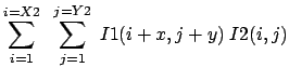
To be able to filter correctly the image, we must know the value of the
background gray level= BGL. This is an iterative algorithm. At each pass,
the value of the BGL is refined. The BGL is calculated using the following
algorithm (s1 is a parameter to give):
|
(1) |
When we calculate the two above average we only use the points that belongs
to the object we want to isolate. A point  does NOT belong to the object if
 . The parameter s2 must be given. The average
are thus calculated on set of points changing at each pass.
. The parameter s2 must be given. The average
are thus calculated on set of points changing at each pass.
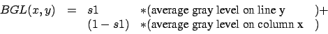
One last pass is done to re-center all the gray level to 128. For each point of the image, we execute:
(new gray level) (old gray level) (old gray level)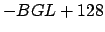 |
(2) |
three parameters used: s3,s4,s5.
Let's consider an image with 3 white peaks. Two of these peaks
belongs to the object to classify, the last one (far away from the
2 others) is noise. We want to crop the image so that only the
object to classify remains.
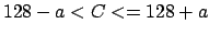
The algorithms begins by searching the point  which has the Gray Level the further away from 128 (128 is now
the color of the background: see previous step: noise cancellation). This
point will usually belong to one of the two peaks evoked before. From
this point we will make a "special flood fill" (see end of the section to
have a more precise description of the flood fill). The program draws a rectangular
box around the zone which has been colored by the "flood fill". Everything
outside this box is cropped.
which has the Gray Level the further away from 128 (128 is now
the color of the background: see previous step: noise cancellation). This
point will usually belong to one of the two peaks evoked before. From
this point we will make a "special flood fill" (see end of the section to
have a more precise description of the flood fill). The program draws a rectangular
box around the zone which has been colored by the "flood fill". Everything
outside this box is cropped.
Ideally, the "flood fill" should color the two right peaks. Unfortunately, there is very often, between these 2 peaks, a zone of the image at 128. This zone prevents the "flood fill" to expand up to the second peaks. To overcome this difficulty, the "flood fill" is executed on a reduced copy of the original image (horizontal scaling:s4, vertical scaling: s5). Based on this colored copy, we crop the original image.
FLOOD FILL: coloring algorithm.
The algorithm start from a given pixel. Then, It colors all the adjacent
pixel. The coloring stops when we find a gray level such that
 with
with
 and
and  =gray level of point .
NOTE: This algorithms works with white or black objects. No problem.
one parameter used: s6.
If the image to classify is still to big, we must crop a little bit more.
We can create a new "cuted" image which contains  (
( should be 90 or 95) of the luminosity of the original image. The
luminosity of an image is defined by the sum of the gray level of all the
points in the image.
should be 90 or 95) of the luminosity of the original image. The
luminosity of an image is defined by the sum of the gray level of all the
points in the image.
The "cutting" algorithm is the following:
 ). of the global luminosity.
four parameters used: s7,s8,s9,s10.
With the toolbox you can easily extract these features (all these in less the 10 ms on a P3 600 MHz):
 . To be less sensitive to the noise, we count the number of peaks
of the curve
. To be less sensitive to the noise, we count the number of peaks
of the curve  with
with
 .. To be less sensitive to the noise, we count the number of peaks
of the curve with
.. To be less sensitive to the noise, we count the number of peaks
of the curve with
 .. To be less sensitive to the noise, we count the number of peaks
of the curve with
.. To be less sensitive to the noise, we count the number of peaks
of the curve with
 .. To be less sensitive to the noise, we count the number of peaks
of the curve with
.. To be less sensitive to the noise, we count the number of peaks
of the curve with
 .
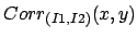
. The correlation of an image  of size
  with an image
  of size
  is an image
  of size
(non-commutativity of the correlation operator).
 and
and
 . )' is the image after a rotation of 180°.
  and
and
 .
.  |
|
 |
(6) |
 |
|
 |
(7) |
 |
|
 |
(8) |
with
 the Fourier transform of the image I.
We have:
 |
|
 |
(9) |
 |
|
 |
(10) |
 = transpose of x.
The convolution operator is a simple multiplication in the Fourier domain.
For each point, we calculate only a single multiplication.
Now, we have
 . we want . We still have to calculate an inverse Fourier Transform:
 |
(11) |
The correlation of two images is available only for images where the gray
level is coded on a double ("ImageD" class). There is a simple function which
creates "ImageD" images from normal images where the gray level is coded in
integer on 8 bits (normal "Image" class).
It's interesting to calculate the correlation of the images that you want
to classify with "prototype" images to see "how close they look like". This
feature is very slow to calculate but it usually contains lots of useful information.
The result of the correlation calculation is an image. From this image, we
will only use (as a feature to inject inside a classifier) the greatest value
of the color of the pixels of .
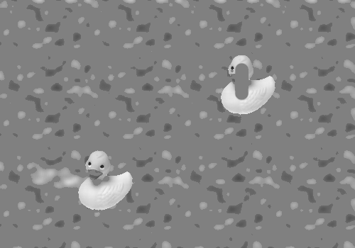
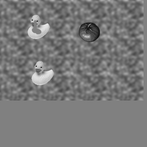
We have an image 'input.png' with noise on it. We want to know if this image
is a duck or a tomato (classification in two classes). We will do a correlation
of the input image with one reference image of a duck ('duck.png') and one
reference image of a tomato ('tomato.png'). The result of this correlation
will be used to determine in with class belong the image 'input.png'.
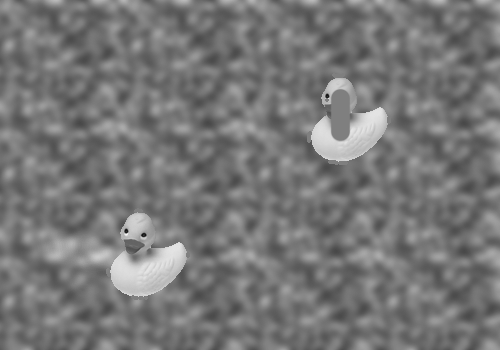 input.png (500x350) |
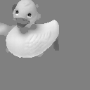
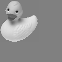
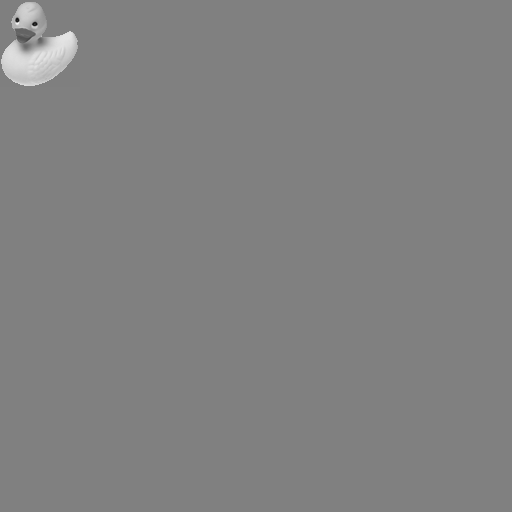
 duck.png (80x87) |
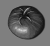 tomato.png (100x93) |
We will first try to remove the noise using the ceiling
technique. We obtain:
'inter0.png'
(500x350)
after ceiling
Everything which was near the "neutral" background gray level 128 has been rounded to 128. We will now isolate the only object of interest in this image (later we will compare this object with the 2 reference objects). We will use a cropping technique.
 'inter1.png' (250x175) The "flood fill" has covered all the object of interest. We will only take the part of the image covered by the flood fill |
 'inter2.png' (150x85) After cropping we have isolated the object to classify |
The size of the image is still too big. A big part of the image is noise. We will apply the second cropping technique

'inter3.png'
(84x82)
We are now ready to start the correlation with the reference images (do not forget to pad the images to a size which is a power of two).
 'inter4.png' (128x128) 'inter3.png' after padding |
* |  'corr0.png' (128x128) 'duck.png' after padding |
= |  'corr1.png' (128x128) The correlation of the two previous images |
'inter4.png' (128x128) 'inter3.png' after padding |
* | 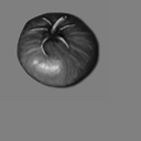 'corr2.png' (128x128) 'tomato.png' after padding |
= |  'corr3.png' (128x128) The correlation of the two previous images |
The correlation between the input image 'input.png' and the reference image
'tomato.png' is 4.956055 (value extracted from 'corr3.png').
The final results is that (hopefully) 'input.png' looks more like a duck than
a tomato (1291.486084>4.956055).
The whole calculation time for the 2 correlations is lower than 80ms on my
P3 600 MHz. Thanks to the FFT algorithm!
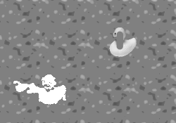
 'inter5.png' (512x512) 'input2.png' after padding |
* |  'corr4.png' (512x512) 'duck.png' after padding |
= 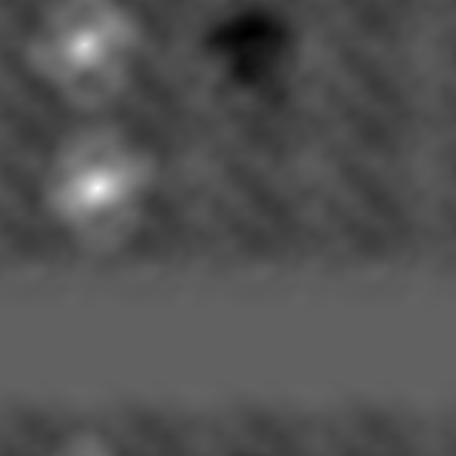 (512x512) |
||
Note the two white spot locatted exacly at the position of the duck inside
'input2.png'. The white spot which is beneath is brighter because the 'input2.png'
ressemble the most at a duck at this position. The emplacement of the tomato
is visible thanks to the black spot.
Calculation time for this correlation is about 3s on my P3 600 MHz.