


Next: Multivariate Lagrange Interpolation
Up: An introduction to the
Previous: The basic trust-region algorithm
Contents
About the CONDOR algorithm.
To start the unconstrained version of the CONDOR algorithm, we
will basically need:
- A starting point

- A length
 which represents, basically, the
initial distance between the points where the objective function
will be sampled.
which represents, basically, the
initial distance between the points where the objective function
will be sampled.
- A length
 which represents, basically, the final
distance between the interpolation points when the algorithm stops.
which represents, basically, the final
distance between the interpolation points when the algorithm stops.
DEFINITION: The local approximation  of
of  is
valid in
is
valid in
 (a ball of radius
  around
 ) when
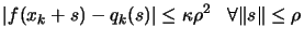 where
where  is a given
constant independent of
is a given
constant independent of  .
.
We will approximatively use the following algorithm (for a
complete description, see chapter 6):
- Create an interpolation polynomial
 of degree 2
which intercepts the objective function around . All
the points in the interpolation set
of degree 2
which intercepts the objective function around . All
the points in the interpolation set  (used to build
 ) are separated by a distance of approximatively
. Set
) are separated by a distance of approximatively
. Set  the best point of the objective
function known so far. Set
the best point of the objective
function known so far. Set
 . In the
following algorithm, is the quadratical approximation of
around , built by interpolation using (see
chapter 3).
. In the
following algorithm, is the quadratical approximation of
around , built by interpolation using (see
chapter 3).
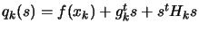 where
where  is the approximate gradient of evaluated at
and
is the approximate gradient of evaluated at
and  is the approximate Hessian matrix of
evaluated at .
is the approximate Hessian matrix of
evaluated at .
- Set

- Inner loop: solve the problem for a given precision of
 .
.
- Solve
 subject to
 .
.
- If
 , then break and go to step
3(b) because, in order to do such a small step, we need to be sure
that the model is valid.
, then break and go to step
3(b) because, in order to do such a small step, we need to be sure
that the model is valid.
- Evaluate the function at the new position
 .
Update the trust region radius
.
Update the trust region radius  and the current best
point using classical trust region technique (following a
scheme similar to Equation 2.20). Include the new
inside the interpolation set . Update to
interpolate on the new .
and the current best
point using classical trust region technique (following a
scheme similar to Equation 2.20). Include the new
inside the interpolation set . Update to
interpolate on the new .
- If some progress has been achieved (for example,
 or there was a reduction
 ),
increment k and return to step i, otherwise continue.
),
increment k and return to step i, otherwise continue.
- Test the validity of
 in
, like
described in chapter 3.
in
, like
described in chapter 3.
- Model is invalid:
Improve the quality of the model
: Remove the worst point of the interpolation set
and replace it (one evaluation required!) with a new point
 such that:
 and the
precision of is substantially increased.
and the
precision of is substantially increased.
- Model is valid:
If
 go back to
step 3(a), otherwise continue.
go back to
step 3(a), otherwise continue.
- Reduce since the optimization steps are
becoming very small, the accuracy needs to be raised.
- If
 stop, otherwise increment k and go back
to step 2.
stop, otherwise increment k and go back
to step 2.
From this description, we can say that and are
two trust region radius (global and local).
Basically, is the distance (Euclidian distance) which
separates the points where the function is sampled. When the
iterations are unsuccessful, the trust region radius
decreases, preventing the algorithm to achieve more progress. At
this point, loop 3(a)i to 3(a)iv is exited and a function
evaluation is required to increase the quality of the model (step
3(b)). When the algorithm comes close to an optimum, the step size
becomes small. Thus, the inner loop (steps 3(a)i. to 3(a)iv.) is
usually exited from step 3(a)ii, allowing to skip step 3(b)
(hoping the model is valid), and directly reducing in
step 4.
The most inner loop (steps 3(a)i. to 3(a)iv.) tries to get from
good search directions without doing any evaluation to
maintain the quality of (The evaluations that are
performed on step 3(a)i) have another goal). Only inside step
3(b), evaluations are performed to increase this quality (called a
''model step'') and only at the condition that the model has
been proven to be invalid (to spare evaluations!).
Notice the update mechanism of in step 4. This update
occurs only when the model has been validated in the trust region
(when the loop 3(a) to 3(b) is exited). The
function cannot be sampled at point too close to the current point
without being assured that the model is valid in
.
The different evaluations of are used to:
- (a)
- guide the search to the minimum of (see inner
loop in the steps 3(a)i. to 3(a)iv.). To guide the search, the
information gathered until now and available in is
exploited.
- (b)
- increase the quality of the approximator (see
step 3(b)). To avoid the degeneration of , the search
space needs to be additionally explored.
(a) and (b) are antagonist objectives like usually the case in the
exploitation/exploration paradigm. The main idea of the
parallelization of the algorithm is to perform the
exploration on distributed CPU's. Consequently, the algorithm
will have better models of at disposal and choose
better search direction, leading to a faster convergence.
CONDOR falls inside the class of algorithm which are proven to be
globally convergent to a local (maybe global) optimum [CST97,CGT00b].
In the next chapters, we will see more precisely:
- Chapter 3: How to construct and use ? Inside the
CONDOR algorithm we need a polynomial approximation of the
objective function. How do we build it? How do we use and validate
it?
- Chapter 4: How to solve
 subject to
 ? We need to know how to solve this
problem because we encounter it at step (3)(a)i. of the CONDOR
algorithm.
? We need to know how to solve this
problem because we encounter it at step (3)(a)i. of the CONDOR
algorithm.
- Chapter 5: How to solve approximately
 subject to
 ? We need to know how to solve this problem because we encounter
it when we want to check the validity (the precision) of the
polynomial approximation.
? We need to know how to solve this problem because we encounter
it when we want to check the validity (the precision) of the
polynomial approximation.
- Chapter 6: The precise description of the CONDOR
unconstrained algorithm.
Next: Multivariate Lagrange Interpolation
Up: An introduction to the
Previous: The basic trust-region algorithm
Contents
Frank Vanden Berghen
2004-04-19