![\fbox{\begin{minipage}[t]{\textwidth}
\begin{center}
\huge {
Constrained, Non-li...
...igh computing load,
noisy objective functions.
\par
}\end{center}\end{minipage}}](img5.png)
CONDOR is mostly useful when used in combination with big software simulators
that simulate industrial processes. These kind of simulators are often encountered
in the chemical industry (simulators of huge chemical reactors), in the compressor
and jet- engine industry (simulators of huge radial turbo-compressors), in the
space industry (simulators of the path of a satellite in low orbit around earth),...
These simulators were written to allow the design engineer to correctly estimate
the consequences of the adjustment of one (or many) design variables (or parameters
of the problem). Such softwares very often demands a great deal of computing
power. One run of the simulator can take as much as one or two hours to finish.
Some extreme simulations take a day to complete.
These kind of codes can be used to optimize ``in batch'' the design variables: The research engineer can aggregate the results of the simulation in one unique number which represents the ``goodness'' of the current design (The aggregation process is handled by CONDOR in a specific way that allows to easily do multi-objective optimization). This final number
Here are the assumptions needed to use CONDOR:
CONDOR is able to use several CPU's in a cluster of computers. Different computer
architectures can be mixed together and used simultaneously to deliver a huge
computing power. The optimizer will make simultaneous evaluations of the objective
function
![]()
![]() on the available CPU's to speed up the optimization process.
on the available CPU's to speed up the optimization process.
You will never loose one evaluation anymore! Why always throwing away the
results of costly evaluations of the objective function? CONDOR manage transparently
a database of old evaluations. Using this database, CONDOR is able to ``hot
start'' very near the optimum point. This proximity ensure rapid convergence.
CONDOR uses the database of old evaluation and a special aggregation process
in a way that allows design engineers to easily ``play'' with the different
sub-objectives without loosing time. Design engineers can easily customize the
objective function, until it finally suits their needs.
The experimental results of CONDOR [VB04] are very encouraging and validates
the quality of the approach: CONDOR outperforms many commercial, high-end optimizer
and it might be the fastest optimizer in its category (fastest in terms of number
of function evaluations). When several CPU's are used, the performances of CONDOR
are unmatched. When performing multi-objective optimization, the possibility
to ``hot start'' near the optimum point allows to converge to the optimum even
faster.
The experimental results open wide possibilities in the field of noisy and
high-computing-load objective function optimization (from two minutes to several
days) like, for instance, industrial shape optimization based on CFD (computation
fluid dynamic) codes (see [CAVDB01,PVdB98,Pol00,PMM$^+$03]) or PDE (partial differential equations)
solvers.
More specifically, in the field of aerodynamic shape optimization, optimizers
based on genetic algorithm (GA) and Artificial Neural Networks (ANN) are very
often encountered. When used on such problems, CONDOR usually outperforms all
the state-of-the-art optimizers based on GA and ANN by a factor of 10 to 100
(see [PPGC04] for classical performances of GA+NN
optimizer). In brief, CONDOR will converge to the solution of the optimization
problem in a time which is 10 to 100 times shorter than any GA+NN optimizers.
When the dimension of the search space increases, the performances of optimizers
based on GA and ANN are drastically dropping. When using a GA+NN optimizer,
a problem with a search-space dimension greater than three is already nearly
unsolvable if the objective function is high-computing-load (All what you can
expect is a slight improvement of the value of the objective function compared
to the value of the objective function at the starting point). Unlike all GA+ANN
optimizers, CONDOR scales very well when the search space dimension increases
(at least up to 100 dimensions).
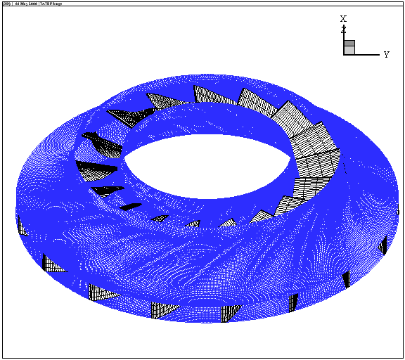
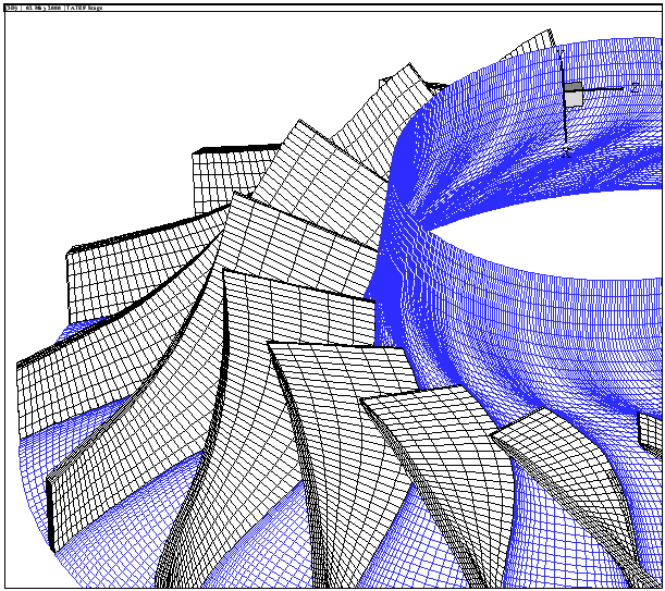
CONDOR has been designed with one application in mind: the METHOD project.
(METHOD stands for Achievement Of Maximum Efficiency For Process Centrifugal
Compressors THrough New Techniques Of Design). The goal of this project is to
optimize the shape of the blades inside a Centrifugal Compressor (see illustration
of the compressor's blades in Figure 1.1).
The objective function is based on a CFD (computation fluid dynamic) code which
simulates the flow of the gas inside the compressor. The shape of the blades
in the compressor is described by 31 parameters. CONDOR is currently the only
optimizer which can solve this kind of problem (an optimizer based on GA+ANN
is useless due to the high number of dimensions and the huge computing time
needed at each evaluation of the objective function). We extract from the numerical
simulation the outlet pressure, the outlet velocity, the energy transmit to
the gas at stationary conditions. We aggregate all these indices in one general
overall number representing the quality of the turbine. We are trying to find
the optimal set of 31 parameters for which this quality is maximum. The evaluations
of the objective function are very noisy and often take more than one hour to
complete (the CFD code needs time to ``converge'').
Finally, The code of CONDOR is completely new, original, easily comprehensible
(Object Oriented approach in C++), (partially) free and fully stand-alone. There
is no call to fortran, external, unavailable, expensive, copyrighted libraries.
You can compile the code under Unix, Windows, Solaris,etc. The only library
needed is the standard TCP/IP network transmission library based on sockets
(only in the case of the parallel version of the code).
The algorithms used inside CONDOR are part of the Gradient-Based optimization
family. The algorithms implemented are Dennis-Moré Trust Region steps calculation
(It's a restricted Newton's Step), Sequential Quadratic Programming (SQP), Quadratic
Programming(QP), Second Order Corrections steps (SOC), Constrained Step length
computation using ![]() merit function and Wolf condition, Active Set method for active
constraints identification, BFGS update, Multivariate Lagrange Polynomial Interpolation,
Cholesky factorization, QR factorization and more! For more in depth information
about the algorithms used, see my thesis [VB04]
merit function and Wolf condition, Active Set method for active
constraints identification, BFGS update, Multivariate Lagrange Polynomial Interpolation,
Cholesky factorization, QR factorization and more! For more in depth information
about the algorithms used, see my thesis [VB04]
Many ideas implemented inside CONDOR are from Powell's UOBYQA (Unconstrained Optimization BY quadratical approximation) [Pow00] for unconstrained, direct optimization. The main contribution of Powell is equation 1.1 which allows to construct a full quadratical model of the objective function in very few function evaluations (at a low price).
 |
(1.1) |
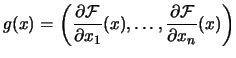
From the user point of view, there are two operating modes available:
CONDOR is an optimizer for non-linear continuous objective functions
subject to box, linear and non-linear constraints. We want to find
![]()
![]()
![]() which satisfies:
which satisfies:
 |
(1.2) |
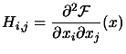
Conventions
|
|
The objective function. We search for the minimum of it. |
| the dimension of the search space | |
| the box-constraints. | |
|
|
the linear constraints. |
| the non-linear constraints. | |
| The optimum of
|
|
| The iteration index of the algorithm | |
| The current point (best point found) | |
 |
|
|
|
|
 |
|
|
|
The Hessian Matrix of
|
|
|
The current approximation of the Hessian Matrix of F at
point |
|
|
The Hessian Matrix at the optimum point. |
|
|
|
All vectors are column vectors.
An optimization (minimization) algorithm is nearly always based on this simple principle:
Like most optimization algorithms, CONDOR uses, as local model, a polynomial
of degree two. There are several techniques to build this quadratic. CONDOR
uses multivariate lagrange interpolation technique to build its model. This
technique is particularly well-suited when the dimension of the search space
is low (![]() ).
).
Let's rewrite this algorithm, using more standard notations:
Currently, most of the research in optimization algorithms is oriented to
huge dimensional search-space (![]() ). In these algorithms, approximative search directions are
computed. CONDOR is one of the very few algorithms which adopts the opposite
point of view. CONDOR build the most precise local models of the objective function
and computes the most precise steps to reduce at all cost the number of function
evaluations.
). In these algorithms, approximative search directions are
computed. CONDOR is one of the very few algorithms which adopts the opposite
point of view. CONDOR build the most precise local models of the objective function
and computes the most precise steps to reduce at all cost the number of function
evaluations.
The material of this chapter is based on the following references: [VB04,Fle87,PT95,BT96,Noc92,CGT99,DS96,CGT00,Pow00].
A (very) basic explanation of the CONDOR algorithm is:
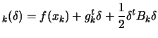
| (1.3) |
 |
(1.4) |
 |
(1.5) |
The local model
![]()
![]() allows us to compute the steps
allows us to compute the steps ![]() which we will follow towards the minimum point
which we will follow towards the minimum point ![]() of
of
![]()
![]() . To which extend can we ``trust'' the local model
. To which extend can we ``trust'' the local model
![]() ? How ``big'' can be the steps
? How ``big'' can be the steps ![]() ? The answer is: as big as the Trust Region Radius
? The answer is: as big as the Trust Region Radius
![]() : We must have
: We must have
![]() .
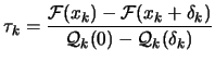
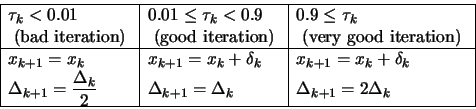
. ![]() is adjusted dynamically at step 5 of the algorithm. The main
idea of step 5 is: only increase
is adjusted dynamically at step 5 of the algorithm. The main
idea of step 5 is: only increase ![]() when the local model
when the local model
![]()
![]() reflects well the real function
reflects well the real function
![]() (and gives us good directions).
(and gives us good directions).
Under some very weak assumptions, it can be proven that this algorithm (Trust
Region algorithm) is globally convergent to a local optimum [CGT00].
To start the unconstrained version of the CONDOR algorithm, we basically need:
There are only a few parameters which have some influence on the convergence speed of CONDOR. We will review them here.
Most people accustomed with finite-difference gradient-based optimization algorithm
are confusing the
![]() or
or ![]() parameters with the
parameters with the ![]() parameter used inside the finite difference formula:
parameter used inside the finite difference formula:
Recalling from step 1 of the algorithm: ``The initial sampling points are
separated by a distance of exactly
![]() ''. If
''. If
![]() is too small, we will build a local approximation
is too small, we will build a local approximation
![]()
![]() which will approximate only the noise inside the evaluations
of the objective function.
which will approximate only the noise inside the evaluations
of the objective function.
What's happening if we start from a point which is far away from the optimum?
CONDOR will make big steps and move rapidly towards the optimum. At each iteration
of the algorithm, we must re-construct
![]()
![]() , the quadratic approximation of
, the quadratic approximation of
![]()
![]() around
around ![]() . To re-construct
. To re-construct
![]()
![]() we will use as interpolating points, old evaluations of
the objective function. Recalling from step 2 of the algorithm: ``The sampling
points are separated from the current point
we will use as interpolating points, old evaluations of
the objective function. Recalling from step 2 of the algorithm: ``The sampling
points are separated from the current point ![]() by a distance of maximum
by a distance of maximum ![]() ''. Thus, if
''. Thus, if ![]() is moving very fast inside the search space and if
is moving very fast inside the search space and if ![]() is small, we will drop many old sampling points because they
are ``too far away''. A sampling point which has been dropped must be replaced
by a new one, requiring a costly evaluation of the objective function.
is small, we will drop many old sampling points because they
are ``too far away''. A sampling point which has been dropped must be replaced
by a new one, requiring a costly evaluation of the objective function.
![]() should thus be chosen big enough to be able to ``move''
rapidly without requiring many evaluations to update/re-construct
should thus be chosen big enough to be able to ``move''
rapidly without requiring many evaluations to update/re-construct
![]()
![]() .
.
![]() represents the average distance between the sample points at
iteration
represents the average distance between the sample points at
iteration ![]() . Above all it represents the ``accuracy'' we want to have when constructing
. Above all it represents the ``accuracy'' we want to have when constructing
![]()
![]() . A small
. A small ![]() will gives us a local model
will gives us a local model
![]()
![]() which represents at very high accuracy the local shape of
the objective function
which represents at very high accuracy the local shape of
the objective function
![]()
![]() . Constructing a very accurate approximation of
. Constructing a very accurate approximation of
![]()
![]() is very costly (for the reason explained in the previous paragraph).
Thus, at the beginning of the optimization process, most of the time, a small
is very costly (for the reason explained in the previous paragraph).
Thus, at the beginning of the optimization process, most of the time, a small
![]() is a bad idea.
is a bad idea.
![]() can be set to a small value only if we start really close
to the optimum point
can be set to a small value only if we start really close
to the optimum point ![]() . See section 1.3.3
to know more about this subject.
. See section 1.3.3
to know more about this subject.
See also the end of section 1.3.4
to have more insight how to choose an appropriate value for
![]() .
.
![]() is the stopping criterion. You should stop once you have
reached the noise level inside the evaluation of the objective function.
is the stopping criterion. You should stop once you have
reached the noise level inside the evaluation of the objective function.
The closer the starting point ![]() is from the optimum point
is from the optimum point ![]() , the better it is.
, the better it is.
If ![]() is far from
is far from ![]() , the optimizer may fall into a local minimum of the objective function.
The objective function encountered in aero-dynamic shape optimization are in
a way ``gentle'': they have usually only one minimum. The difficulty is coming
from the noise inside the evaluations of the objective function and from the
(long) computing time needed for each evaluation.
, the optimizer may fall into a local minimum of the objective function.
The objective function encountered in aero-dynamic shape optimization are in
a way ``gentle'': they have usually only one minimum. The difficulty is coming
from the noise inside the evaluations of the objective function and from the
(long) computing time needed for each evaluation.
Equation 1.3 means that the steps
sizes must be greater than
![]() . Thus, if you start very close to the optimum point
. Thus, if you start very close to the optimum point
![]() (using for example the hot-start functionality of CONDOR), you
should consider to use a very small
(using for example the hot-start functionality of CONDOR), you
should consider to use a very small
![]() otherwise the algorithm will be forced to make big steps
at the beginning of the process. This behavior is easy to identify: it gives
a spiraling path to the optimum.
otherwise the algorithm will be forced to make big steps
at the beginning of the process. This behavior is easy to identify: it gives
a spiraling path to the optimum.
From equation 1.3:
Let's consider the following optimization problem which aims to optimize the
shape of the hull of a boat:
In this example the re-scaling factors are ![]() and
and ![]() .
.
When automatic re-scaling is used, CONDOR will rescale automatically and transparently
the variables to obtain the highest speed. The re-scaling factors ![]() are computed in the following way:
are computed in the following way:
![]() . If some bounds constrained (
. If some bounds constrained (![]() and
and ![]() ) are defined on axis
) are defined on axis ![]() , then
, then
![]() .
.
To obtain higher convergence speed, you can override the auto-rescaling feature
and specify yourself more accurate rescaling factors.
![]() and
and
![]() are distances expressed in the rescaled-space. Usually,
when using auto-rescaling, a good starting value for
are distances expressed in the rescaled-space. Usually,
when using auto-rescaling, a good starting value for
![]() is
is ![]() . This will make the algorithm very robust against noise. Depending
on the noise level and on the experience you have with your objective function,
you may, at a later time, decide to reduce
. This will make the algorithm very robust against noise. Depending
on the noise level and on the experience you have with your objective function,
you may, at a later time, decide to reduce
![]() .
.
The different evaluations of
![]()
![]() are used to:
are used to:
(a) and (b) are antagonist objectives like it is usually the case in the exploitation/exploration
paradigm. The main idea of the parallelization of the algorithm is to perform
the exploration on distributed CPU's. Consequently, the algorithm will
have better models
![]()
![]() of
of
![]()
![]() at its disposal and choose better search directions, leading to
a faster convergence.
at its disposal and choose better search directions, leading to
a faster convergence.
When the dimension of the search space is low, there is no need to make many
samples of
![]()
![]() to obtain a good approximation
to obtain a good approximation
![]()
![]() . Thus, the parallel algorithm is more useful for large dimension
of the search space.
. Thus, the parallel algorithm is more useful for large dimension
of the search space.
The CONDOR optimizer is taking as parameter on the command-line the name of a XML file containing all the required information needed to start the optimization process.
Let's start with a simple example:
<?xml version="1.0" encoding="ISO-8859-1"?>
<configCONDOR>
    <!--  name of all design variables (tab separated) -->
    <varNames dimension="4">
        x1 x2 x3 x4
    </varNames>

    <objectiveFunction nIndex="5">

         <!--- name of the outputs which are computed by the
          simulator. If not enough names are given, the same
          names are used many times with a different prefixed
          number (tab separated) -->
        <indexNames>
             indexA indexB
        </indexNames>

        <!-- the aggregation function -->
        <aggregationFunction>

              indexA_1+indexB_1+indexA_2+indexB_2+indexA_3

              <!-- if there are several sub-objective,
              specify them here:
              <subAggregationFunction name="a">
              </subAggregationFunction> -->

        </aggregationFunction>

        <!-- blackbox objective function -->
        <executableFile>
             OF/testOF
        </executableFile>

        <!-- objective function: input file -->
        <inputObjectiveFile>
            optim.out
        </inputObjectiveFile>

        <!-- objective function: output file -->
        <outputObjectiveFile>
            simulator.out
        </outputObjectiveFile>

        <!-- optimization of only a part of the variables -->
        <variablesToOptimize>
            <!-- 1  2  3  4   -->
                 1  1  1  1
        </variablesToOptimize>
    </objectiveFunction>

    <!-- a priori estimated x (starting point) -->
    <startingPoint>
    <!--    1      2    3    4  -->
         -1.2   -1.0   -1    3
    </startingPoint>

    <constraints>
        <!-- lower bounds for x -->
        <lowerBounds>
            <!--
              1   2   3   4 -->
            -10 -10 -10 -10
        </lowerBounds>

        <!-- upper bounds for x -->
        <upperBounds>
            <!--
             1  2  3  4 -->
            10 10 10 10
        </upperBounds>

        <!-- Here would be the matrix for linear
             inequalities definition if they were needed
        <linearInequalities>
            <eq>
            </eq>
        </linearInequalities> -->

        <!-- non-Linear Inequalities
        <nonLinearInequalities>
            <eq>
            </eq>
        </nonLinearInequalities> -->

        <!-- non-Linear equalities
        <equalities>
            <eq>
            </eq>
        </equalities> -->
    </constraints>

    <!-- scaling factor for the normalization of
         the variables (optional) -->
    <scalingFactor auto />

    <!-- parameter for optimization:
          *rho_start: initial distance between
               sample sites (in the rescaled space)
          *rho_end: stopping criteria(in the
               rescaled space)
          *timeToSleep: when waiting for the result
               of the evaluation of the objective
               function, we check every xxx seconds
               for an appearance of the file containing
               the results (in second).
          *maxIteration: maximum number of iteration
    -->
    <optimizationParameters
        rhostart    =".1  "
        rhoend      ="1e-3"
        timeToSleep =".1  "
        maxIteration="1000"
    />

    <!-- all the datafile are optional:
       *binaryDatabaseFile: the filename of the full
            DB data (WARNING!! BINARY FORMAT!)
       *asciiDatabaseFile: data to add to the full DB
            data file (in ascii format)
       *traceFile: the data of the last run are inside
            a file called? (WARNING!! BINARY FORMAT!) -->
    <dataFiles
        binaryDatabaseFile="dbEvalsQ4N.bin"
        asciiDatabaseFile="dbEvalsQ4N.txt"
        traceFile="traceQ4N.bin"
    />

    <!-- name of the save file containing the end
         result of the optimization process -->
    <resultFile>
        traceQ4N.txt
    </resultFile>

    <!-- the sigma vector is used to compute sensibilities
         of the Obj.Funct. relative to variation of
         amplitude sigma_i on axis i -->
    <sigmaVector>
        1 1 1 1
    </sigmaVector>

</configCONDOR>
All the extra tags which are not used by CONDOR are simply ignored. You can
thus include additional information inside the configuration file without any
problem (it's usually better to have one single file which contains everything
which is needed to start an optimization run). The full path to the XML file
is given as first command-line parameter to the executable which evaluates the
objective function.
The varNames tag describes the name of the variables we want to optimize. These variables will be referenced thereafter as design variables. These are three equivalent definitions of the same design variable names:
<varNames dimension="2" />
<varNames> X_01 X_02 </varNames>
<varNames dimension="2"> X_01 X_02 </varNames>
In the last case, the dimension attribute and the number of name given
inside the varNames tag must match. When giving specific name, each name
is separated from the next one by either a space, a tabulation or a carriage return
(unix,windows). The varNames tag also describes what's the dimension
of the search space. Let's define The objectiveFunction tag describes the objective function. Usually,
each evaluation of the objective function is performed by an external executable.
The name of this executable is specified in the tag executableFile.
This executable takes as input a file which contains the point where the objective
function must be evaluated. The name of this file is specified in the tag inputObjectiveFile.
In return, the executable write the result of the evaluation inside a file specified
in the tag outputObjectiveFile. When CONDOR runs the executable, it
gives three extra parameters on the command-line: the full path to the XML-configuration
file, the inputObjectiveFile and the outputObjectiveFile.
The result file outputObjectiveFile contains a vector ![]() of numbers called index variables.
of numbers called index variables.
There are 2 ways to specify the dimension of ![]() :
:
    <objectiveFunction nIndex="3">
        ...
    <objectiveFunction>
        <indexNames> Y_001 Y_002 Y_003 </indexNames>
        ...
These are two equivalent definition of the same six index variable names:
    <objectiveFunction nIndex="6">
        <indexNames> U V </indexNames>
        ...
    <objectiveFunction>
        <indexNames> U_1 V_1 U_2 V_2 U_3 V_3 </indexNames>
        ...
Suppose you want to optimize a seal design. For a seal optimization, we want to minimize the leakage at low speed and high pressure(1), minimize the efficiency-loss due to friction at high speed(2), maximize the ``lift'' at low speed and low pressure(3). The overall quality of a specific design of a seal, we will be computed based on 3 different simulations of the same seal design at the following three operating point: low speed and high pressure(1), high speed(2), low speed and low pressure(3). Suppose each run of the simulator gives as result four index variables: A,B,C,D. We will have the following XML configuration (the content of the aggregationFunction tag will be explained hereafter):
    ...
    <objectiveFunction nIndex="12">
        <indexNames> A B C D </indexNames>
        <aggregationFunction>
              <subAggregationFunction name="leakage">
                  <!-- compute the leakage based on A_1, B_1, C_1, D_1 -->
                  5*(A_1^3)
              </subAggregationFunction>
              <subAggregationFunction name="friction_loss">
                  <!-- compute the efficiency loss due to friction
                       based on A_2, B_2, C_2, D_2 -->
                  2.1*(-B_1^2+C_1^2)
              </subAggregationFunction>
              <subAggregationFunction name="lift">
                  <!-- compute the ``lift'' based on A_3, B_3, C_3, D_3 -->
                  0.5*(sqrt(D_3))
              </subAggregationFunction>
        </aggregationFunction>
        ...
All the values of the index variables) must be aggregated into one
number which will be optimized by CONDOR. The aggregation function is given
in the tag
aggregationFunction. If this tag is missing, CONDOR will use as aggregation
function the sum of all the index variables.
You can define inside the tag aggregationFunction, some sub-objectives.
Each sub-objective is defined inside the tag subAggregationFunction.
The tag subAggregationFunction can have an optional parameter name
which will appear inside the tracefile. The global aggregation function
is the sum of all the sub-objectives. You can look inside the trace-file of
the optimization process to see how the different subobjectives are comparing
together and adjust accordingly the equations defining the subobjectives. Typically,
this procedure is iterative: you define some approximate sub-objectives functions,
you run CONDOR, you observe ``where'' CONDOR is heading for, you look inside
the trace file to see what's the reason of such direction, you adjust the different
sub-objectives giving more or less weight to specific sub-objectives and you
restart CONDOR, etc.
The aggregationFunction tag or the subAggregationFunction
tag contains simple equations which can have as ``input variables'' all the
design variables and all the index variables. The mathematical
operators that are allowed are:
![]() ,
, ![]() (base:
(base:![]() ),
), ![]() ,
, ![]() ,
, ![]() ,
, ![]() ,
, ![]() ,
, ![]() ,
, ![]() ,
, ![]() ,
, ![]() ,
, ![]() ,
, ![]() ,
, ![]() ,
, ![]() ,
, ![]() ,
, ![]() ,
, ![]() ,
, ![]() ,
, ![]() .
.
In the example above (about seal design), the sub-objectives are the leakage,
the efficiency-loss due to friction and the ``lift''. The weights of the different
sub-objectives have been adjusted to respectively 5, 2.1 and 0.5 by the design
engineer. The values of the index variables A_1, B_1, C_1, D_1,
A_2, B_2, C_2, D_2, A_3, B_3, C_3, D_3 for all the different computed seal
designs have been saved inside the database of CONDOR and can be re-used to
``hot-start'' CONDOR. The initialization phase of CONDOR is usually time consuming
because we need to compute many samples of the objective function
![]()
![]() to build the first
to build the first
![]()
![]() ). The initialization phase can be strongly shortened using
the ``hot-start''.
). The initialization phase can be strongly shortened using
the ``hot-start''.
If none of the aggregation functions and none of the sub-aggregation functions
are using any index variables, you can omit the indexNames,
executableFile, inputObjectiveFile and outputObjectiveFile
tags. You can also omit the nIndex attribute of the objectiveFunction
tag and the timeToSleep attribute of the optimizationParameters
tag. The attributes binaryDatabaseFile and asciiDatabaseFile
of the dataFiles tag are ignored. This feature in mainly useful for
quick demonstration purposes.
The variablesToOptimize tag defines which design variables CONDOR
will optimize. This tag contains a vector ![]() of dimension
of dimension ![]() (
(
![]() ). If
). If ![]() equals 0 the design variable of index
equals 0 the design variable of index ![]() will not be optimized.
will not be optimized.
The startingPoint tag defines what's the starting point. It contains
a vector ![]() of dimension
of dimension ![]() . If this tag is missing, CONDOR will use as starting point the best
point found inside its database. If the database is empty, then CONDOR issues
an error and stops.
. If this tag is missing, CONDOR will use as starting point the best
point found inside its database. If the database is empty, then CONDOR issues
an error and stops.
The constraints tag defines what are the constraints. It's an optional tag. It contains the tags lowerBounds and upperBounds which are self explanatory. It also contains the tag linearInequalities which describes linear inequalities. If the feasible space is described by the following three linear inequalities:
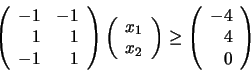
    <constraints>
        <linearInequalities>
        -1 -1 -4
         1  1  4
        -1  1  0
        </linearInequalities>
        ...
or by:
    <constraints>
        <linearInequalities>
             <eq> -1 -1 -4 </eq>
             <eq>  1  1  4 </eq>
             <eq> -1  1  0 </eq>
        </linearInequalities>
        ...
A carriage return or a <eq>..</eq> tag pair is needed to
separate each linear inequality. The two notations cannot be mixed. The constraints
tag also contains the nonLinearInequalities tag which describes non linear
inequalities
    ...
    <varNames> x0 x1 </varNames>
    ...
    <constraints>
        <nonLinearInequalities>
            <eq> 1-x0*x0-x1*x1 </eq>
            <eq> -x0*x0+x1      </eq>
        </nonLinearInequalities>
        ...
If there is only one non-linear inequality, you can write it directly, without
the eq tags. CONDOR also handles a primitive form of equality constraints.
The equalities must be given in an explicit way. For example:
    ...
    <varNames> x0 x1 x2 </varNames>
    <constraints>
        <equalities> x2=(1-x0)^2 </equalities>
        ...
(the <eq>...</eq> tag pair has been omitted because there
is only one equality). The re-scaling factors
![]() are defined inside the scalingFactor tag. For more information
about the re-scaling factors, see section 1.3.4.
If the re-scaling factors are missing, CONDOR assumes
are defined inside the scalingFactor tag. For more information
about the re-scaling factors, see section 1.3.4.
If the re-scaling factors are missing, CONDOR assumes
![]() . To have automatic computation of the re-scaling factors, write:
. To have automatic computation of the re-scaling factors, write:
<scalingFactor auto/>
The optimizationParameters tag contains the following attributes:
The dataFiles tag contains the following attributes:
The name of the file containing the end result of the optimization process
is given inside the resultFile tag. This is an ascii file which contains:
the dimension of search-space, the total number of function evaluation (total
NFE), the number of function evaluation before finding the best point, the value
of the objective function at solution, the solution vector ![]() , the Hessian matrix at the solution
, the Hessian matrix at the solution ![]() , the gradient vector at the solution
, the gradient vector at the solution ![]() (it should be zero if there is no active constraint), the lagrangian
Vector at the solution (for lower,upper,linear,non-linear constraints), the
sensitivity vector.
(it should be zero if there is no active constraint), the lagrangian
Vector at the solution (for lower,upper,linear,non-linear constraints), the
sensitivity vector.
The sigma vector which is used to compute sensibilities of the Objective Function
relatively to variation of amplitude ![]() on axis
on axis ![]() is given inside the sigmaVector tag.
is given inside the sigmaVector tag.
This file contains the point
![]() where the objective function must be evaluated. It's an
ascii file containing only one line. This line contains all the component
where the objective function must be evaluated. It's an
ascii file containing only one line. This line contains all the component ![]() of
of ![]() separated by a tabulation. The inputObjectiveFile is given
as second command-line parameter to the executable which evaluates the objective
function.
separated by a tabulation. The inputObjectiveFile is given
as second command-line parameter to the executable which evaluates the objective
function.
This file can be ascii or binary. If the first byte of the file is 'A' then the file will be ascii. If the first byte of the file is 'B' then the file will be binary. The outputObjectiveFile is given as third command-line parameter to the executable which evaluates the objective function.
The file contains at least 3 lines:
The structure is the following:
The binaryDatabaseFile is a simple matrix stored in binary format.
Each line corresponds to an evaluation of the objective function. You will find
on a line all the design variables followed by all the index variables
(![]() numbers).
numbers).
The utility 'matConvert.exe' converts a full precision binary matrix file
to an easy manipulating matrix ascii files.
The structure of the binary matrix file is the following:
The asciiDatabaseFile is a simple matrix stored in ascii format.
Each line of the matrix corresponds to an evaluation of the objective function.
You will find on a line all the design variables followed by all the
index variables. (![]() numbers)
numbers)
The utility 'matConvert.exe' converts a full precision binary matrix file
to an easy manipulating matrix ascii files.
The structure of the ascii matrix file is the following:
The traceFile is a simple matrix stored in binary format. The utility 'matConvert.exe' converts a full precision binary matrix file to an easy manipulating matrix ascii files. Each line of the matrix corresponds to an evaluation of the objective function. You will find on a line:
Most of the time, when researchers are confronted to a noisy optimization problem, they are using an algorithm which is a combination of Genetic Algorithm and Neural Network. This algorithm will be referred in the following text under the following abbreviation: (GA+NN). The principle of this algorithm is the following:
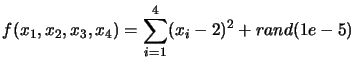
A xml-configuration file for the standard case is given in section 2.1. You can run this example with the script file named 'testQ4N'. The objective function is computed in an external executable and is:
The script-file named 'testQ4N' optimizes the same objective function but, this time, without noise. Using CONDOR we obtain:
The xml-configuration file for this example is given is section 2.1.
The content of the tag executableFile needs to be changed: it must
be replace by "OF/testOFF". You can run this example with the script file named
'testQ4NF'. The objective function is the same as in the previous subsection:
a simple 4 dimensional quadratic centered at ![]() and perturbated with a noise of maximum amplitude
and perturbated with a noise of maximum amplitude ![]() . The failure are simulated using a random number:
. The failure are simulated using a random number:
if rand(1.0)>.55 then fail else succeed.
The evaluation of the objective function at the given starting point cannot
fail. If this happens, CONDOR has no starting point and it stops immediately.
The xml-configuration file for this example is the following:
<?xml version="1.0" encoding="ISO-8859-1"?>
<configCONDOR>
    <varNames> x_1 x_2 </varNames>
    <objectiveFunction>
        <aggregationFunction>
            100*(x_2-x_1^2)^2+(1-x_1)^2
        </aggregationFunction>
    </objectiveFunction>
    <startingPoint> -1.2   -1.0 </startingPoint>
    <constraints>
        <lowerBounds> -10 -10 </lowerBounds>
        <upperBounds>  10 10  </upperBounds>
    </constraints>
    <optimizationParameters
        rhostart    =" 1    "
        rhoend      =" 1e-2 "
        maxIteration=" 1000 "
    />
    <dataFiles traceFile="traceRosen.dat" />
    <resultFile> resultsRosen.txt </resultFile>
    <sigmaVector> 1 1 </sigmaVector>
</configCONDOR>
You can run this example with the script file named 'testRosen'. In the optimization
community this function is a classical test-case. The minimum of the function
is at 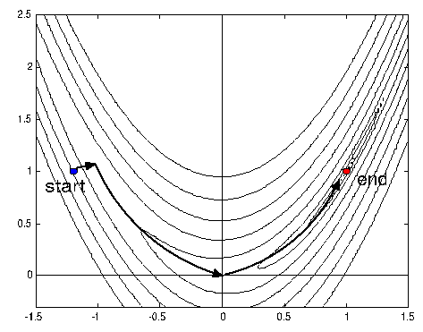 |
For optimizers which are following the slope (like CONDOR), this function is a real challenge. In opposition, (GA+NN) optimizers are not using the concept of slope and should not have any special difficulties to find the minimum of this function. Beside (GA+NN) are most efficient on small dimensional search space (in opposition to CONDOR). They should thus exhibit very good performances compared to CONDOR on this problem. Using CONDOR we obtain:
In the previous subsection, we have seen that the performances of CONDOR on the Rosenbrock function are low because the optimizer must avoid a ``barrier'' inside the objective function before it can ``home'' to the minimum. What happens if we remove this barrier? Let's consider the following xml-configuration file:
<?xml version="1.0" encoding="ISO-8859-1"?>
<configCONDOR>
    <varNames> x_0 x_1 </varNames>
    <objectiveFunction>
        <aggregationFunction>  (x_1-2)^2+(x_0-2)^2   </aggregationFunction>
    </objectiveFunction>
    <startingPoint> 0   0 </startingPoint>
    <constraints>
        <lowerBounds> -10 -10 </lowerBounds>
        <upperBounds>  10  10 </upperBounds>
    </constraints>
    <scalingFactor auto/>
    <optimizationParameters
        rhostart    =" 1    "
        rhoend      =" 9e-1 "
        maxIteration=" 1000 "
    />
    <dataFiles traceFile="traceQ2.dat" />
    <resultFile> resultsQ2.txt </resultFile>
    <sigmaVector> 1 1 </sigmaVector>
</configCONDOR>
You can run this example with the script file named 'testQ2'. Using CONDOR we
obtain:
The xml-configuration file for this example is the following:
<?xml version="1.0" encoding="ISO-8859-1"?>
<configCONDOR>
    <varNames> x0 x1 </varNames>
    <objectiveFunction>
        <aggregationFunction>
            100*(x1/1000-x0^2)^2+(1-x0)^2
        </aggregationFunction>
    </objectiveFunction>
    <startingPoint> -1.2   -1000 </startingPoint>
    <constraints>
        <lowerBounds> -10 -10000 </lowerBounds>
        <upperBounds>  10  10000  </upperBounds>
    </constraints>
    <scalingFactor auto/>
    <optimizationParameters
        rhostart    =" .1    "
        rhoend      =" 1e-5 "
        maxIteration=" 1000 "
    />
    <dataFiles traceFile="traceScaledRosen.dat"  />
    <resultFile> resultsScaledRosen.txt </resultFile>
    <sigmaVector> 1 1 </sigmaVector>
</configCONDOR>
You can run this example with the script file named 'testScaledRosen'. As explained in section 1.3.4, the design variables x0 and x1 must be in the same order of magnitude to obtain high convergence speed. This is not the case here: x1 is 1000 times greater than x0. Some appropriate re-scaling factors are computed by CONDOR and applied. Using CONDOR we obtain:
One technique to deal with linear and box constraints is the ``Gradient Projection
Methods''. In this method, we follow the gradient of the objective function.
When we enter the infeasible space, we will simply project the gradient into
the feasible space. The convergence speed of this algorithm is, at most, linear,
requiring many evaluation of the objective function.
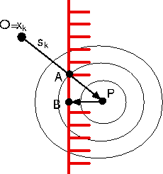
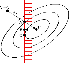
A straightforward (unfortunately false) extension to this technique is the ``Newton Step Projection Method''. This technique should allow (if it works) a very high (quadratical) speed of convergence. It is illustrated in figure 2.3. This method is the following:
In figure 2.3, the current point is
![]() . The Newton step (
. The Newton step (![]() ) lead us to point P which is infeasible. We project P into
the feasible space: we obtain B. Finally, we will thus follow the trajectory
OAB, which seems good.
) lead us to point P which is infeasible. We project P into
the feasible space: we obtain B. Finally, we will thus follow the trajectory
OAB, which seems good.
In figure 2.4, we can see that the
"Newton step projection algorithm" can lead to a false minimum. As before, we
will follow the trajectory OAB. Unfortunately, the real minimum of the problem
is C.
Despite its wrong foundation, the ``Newton Step Projection Method'' is very
often encountered [BK97,Kel99,SBT$^+$92,GK95,CGP$^+$01]. CONDOR uses an other technique based
on active-set method which allows very high (quadratical) speed on convergence
even when ``sliding'' along a constraint.
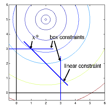
Let's have a small example:
<?xml version="1.0" encoding="ISO-8859-1"?>
<configCONDOR>
    <varNames> x0 x1 </varNames>
    <objectiveFunction>
        <aggregationFunction>   (x0-2)^2+(x1-5)^2    </aggregationFunction>
    </objectiveFunction>
    <startingPoint> 0  0 </startingPoint>
    <constraints>
        <lowerBounds>   -2 -3  </lowerBounds>
        <upperBounds>    3  3  </upperBounds>
        <linearInequalities>
            <eq>   -1   -1   -4 </eq>
        </linearInequalities>
    </constraints>
    <scalingFactor auto/>
    <optimizationParameters
        rhostart    =" 1    "
        rhoend      =" 1e-2 "
        maxIteration=" 1000 "
    />
    <dataFiles traceFile="traceSuperSimple.dat"    />
    <resultFile>    resultsSuperSimple.txt     </resultFile>
    <sigmaVector>  1 1  </sigmaVector>
</configCONDOR>
You can run this example with the script file named 'testSuperSimple'. This problem is illustrated in figure 2.5. Using CONDOR, we obtain
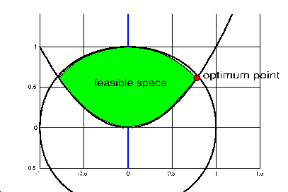
The xml-configuration file for this example is the following:
<?xml version="1.0" encoding="ISO-8859-1"?>
<configCONDOR>
    <varNames> v0 v1 </varNames>
    <objectiveFunction>
        <aggregationFunction>    -v0   </aggregationFunction>
    </objectiveFunction>
    <startingPoint>  0   0  </startingPoint>
    <constraints>
        <!-- non-Linear Inequalities: v is feasible <=> c_i(v)>=0 -->
        <nonLinearInequalities>
            <eq> 1-v0*v0-v1*v1 </eq>
            <eq> v1-v0*v0      </eq>
        </nonLinearInequalities>
    </constraints>
    <optimizationParameters
        rhostart    =" .1   "
        rhoend      =" 1e-6 "
        maxIteration=" 1000 "
    />
    <dataFiles traceFile="traceFletcher.dat"  />
    <resultFile> resultsFletcher.txt  </resultFile>
    <sigmaVector> 1 1 </sigmaVector>
</configCONDOR>
You can run this example with the script file named 'testFletcher'. The feasible space is illustrated in figure 2.6. Using CONDOR, we obtain
[xopt,vopt,lambdaopt,trace]=matlabCondor(rhostart,rhoend,maxIteration,params,optionalParam);The input parameters are:
function [output,error] = ObjFunct(px)
The output parameter error is optional. If the evaluation
has failed then the function must return error=1 . output
is a scalar which contains the value of the objective function f(x)
evaluated at position px.
function [output,error] = NLConstr(isGradNeeded,J,px)
The output parameter error is optional. If isGradNeeded=0,
then output must be a scalar that contains the value of the
JpRosen.xstart=[-1.2 -1.0]; pRosen.f = 'OF_Rosen'; pRosen.lb=[-10-10]; pRosen.ub=[ 10 10]; pRosen.scalingFactor= []; rhostart=1; rhoend=.01; niter=1000;The function OF_Rosen is the following:
function [out,error] = OF_Rosen(x)
out= 100*(x(2)-x(1)^2)^2+(1-x(1))^2;
error=0;
A complete description of this problem is given in section 2.7.3. The .m files used in this examples are 'test_Rosen.m' and 'OF_Rosen.m'.
In preparation.
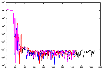
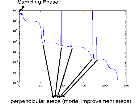
You can see in figure 4.1 a trace of an optimization run of CONDOR. On the x-axis, you have the time
CONDOR always starts by sampling the objective function to build the initial
quadratical approximation
![]()
![]() of
of
![]()
![]() around
around ![]() (see section 1.2 -
step 1: Initialization). This is called the sampling/initial construction
phase. During this phase the optimizer will not follow the slope towards the
optimum. Therefore the values of the objective function remains more or less
the same during all the sampling phase (as you can see in figure 4.1).
Once this phase is finished, CONDOR has enough information to be able to follow
the slope towards the minimum. The information gathered up to now during the
sampling phase are finally used. This is why, usually, just after the end of
the sampling phase, there is a significant drop inside the value of the objective
function (see figure 2.1).
(see section 1.2 -
step 1: Initialization). This is called the sampling/initial construction
phase. During this phase the optimizer will not follow the slope towards the
optimum. Therefore the values of the objective function remains more or less
the same during all the sampling phase (as you can see in figure 4.1).
Once this phase is finished, CONDOR has enough information to be able to follow
the slope towards the minimum. The information gathered up to now during the
sampling phase are finally used. This is why, usually, just after the end of
the sampling phase, there is a significant drop inside the value of the objective
function (see figure 2.1).
This first construction phase requires
![]() evaluations of the objective function (
evaluations of the objective function (![]() is the dimension of the search space). This phase is thus very lengthy.
Furthermore, during this phase, the objective function is usually not ``reduced''.
The computation time can be strongly reduced if you use ``hot start''. Another
possibility to reduce the computation time is to use the parallel version of
CONDOR. This phase can be parallelized very easily and without efficiency-loss.
If you use
is the dimension of the search space). This phase is thus very lengthy.
Furthermore, during this phase, the objective function is usually not ``reduced''.
The computation time can be strongly reduced if you use ``hot start''. Another
possibility to reduce the computation time is to use the parallel version of
CONDOR. This phase can be parallelized very easily and without efficiency-loss.
If you use
![]() computers in parallel the computation time of
the sampling phase will be reduced by
computers in parallel the computation time of
the sampling phase will be reduced by ![]() .
.
From time to time CONDOR is making a ``perpendicular'' or ``model improvement''
step. The aim of this step is to avoid the degeneration of the quadratical approximation
![]()
![]() of
of
![]()
![]() . Thus, when performing a ``model improvement'' step, CONDOR will
not try to follow the slope of the objective function and will produce (most
of the time) a very bad values of
. Thus, when performing a ``model improvement'' step, CONDOR will
not try to follow the slope of the objective function and will produce (most
of the time) a very bad values of
![]()
![]() .
.
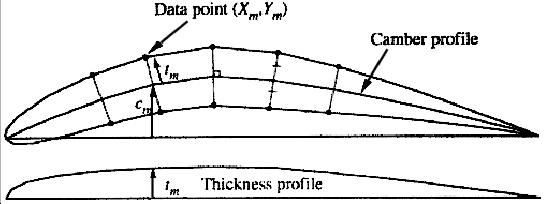
Let's assume you want to optimize a shape. A shape can be parameterized using different tools:
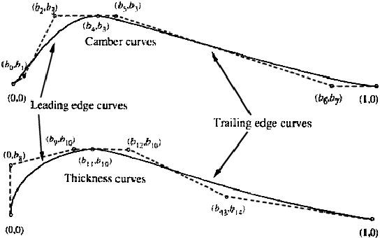
Let's assume we have parameterized the shape of a blade using ``Bezier curves''.
An illustration of the parametrization of an airfoil blade using Bezier curves
is given in figures 4.2 and 4.3.
Some set of shape parameters generates infeasible geometries. The ``feasible
space'' of the constrained optimization problem is defined by the set of parameters
which generates feasible geometries. A good parametrization of the shape to
optimize should only involve box or linear constraints. Non-linear constraints
should be avoided.
In the airfoil example, if we want to express that the thickness of the airfoil
must be non-null, we can simply write
![]() (3 box constraints) (see Figure 4.3
about
(3 box constraints) (see Figure 4.3
about
![]() and
and ![]() ). Expressing the same constraint (non-null thickness) in an
other, simpler, parametrization of the airfoil shape (direct description of
the upper and lower part of the airfoil using 2 bezier curves) can lead to non-linear
constraints. The parametrization of the airfoil proposed here is thus very good
and can easily be optimized.
). Expressing the same constraint (non-null thickness) in an
other, simpler, parametrization of the airfoil shape (direct description of
the upper and lower part of the airfoil using 2 bezier curves) can lead to non-linear
constraints. The parametrization of the airfoil proposed here is thus very good
and can easily be optimized.
 |
If you want, for example, to optimize ![]() variables, never do the following:
variables, never do the following:
This algorithm will results in a very slow linear speed of convergence as illustrated in Figure 4.4. The config-file-parameter variablesToOptimize allows you to activate/deactivate some variables, it's sometime a useful tool but don't abuse from it! Use with care!
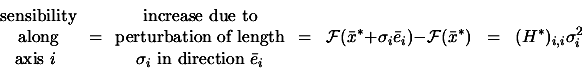
Let's apply a small perturbation ![]() to the optimum point
to the optimum point ![]() in the direction
in the direction ![]() . Let's assume that the objective function is minimum at
. Let's assume that the objective function is minimum at ![]() . How much does this perturbation increase the value of the
objective function?
. How much does this perturbation increase the value of the
objective function?
 |
(4.1) |
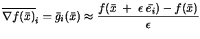
The sigma vector is used to check the sensibilities of the objective function
relative to small perturbation on the coordinates of ![]() . If
. If ![]() represents the optimal design for a shape, the sigma vector help
us to see the impact on the objective function of the manufacturing tolerances
of the optimal shape.
represents the optimal design for a shape, the sigma vector help
us to see the impact on the objective function of the manufacturing tolerances
of the optimal shape.
The same result can be obtained when convoluting the objective function with
a gaussian function which has as variances the ![]() 's.
's.
One of the output CONDOR is giving at the end of the optimization process
is the lagrangian Vector ![]() at the solution. What's useful about this lagrangian vector?
at the solution. What's useful about this lagrangian vector?
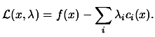
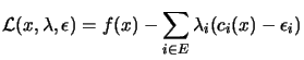
We define the classical Lagrangian function ![]() as:
as:
 |
(4.2) |
 |
(4.3) | |
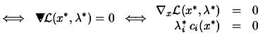
where ![$\displaystyle \begin{picture}(.27,.3) \put(0,0){\makebox(0,0)[bl]{$\nabla$}} \p...
...cture} = \left( \begin{array}{c} \nabla_x \\ \nabla_\lambda \end{array} \right)$](img191.png) |
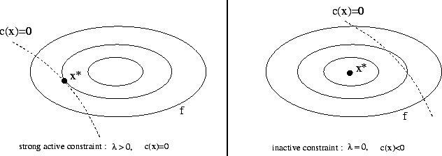
The second equation of 4.3 is called
the complementarity condition. It states that both ![]() and
and ![]() cannot be non-zero, or equivalently that inactive constraints
have a zero multiplier. An illustration is given in figure 4.5.
cannot be non-zero, or equivalently that inactive constraints
have a zero multiplier. An illustration is given in figure 4.5.
 |
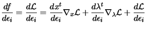
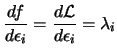
To have some insight into the meaning of Lagrange Multipliers ![]() , consider what happens if the right-hand sides of the constraints
are perturbated, so that
, consider what happens if the right-hand sides of the constraints
are perturbated, so that
| (4.4) |
 |
(4.5) |
 |
(4.6) |
 |
(4.7) |
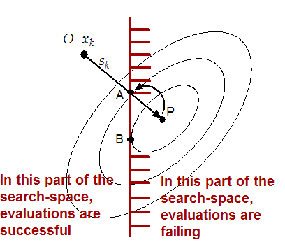
Let's consider figure 4.6 which
is illustrating two consecutive failure (points A and B) inside the evaluation
of the objective function. The part of the search-space where the evaluations
are successful is defined by a ``virtual constraint'' (the red line in figure
4.6). We don't have the equation
of this ``virtual constraint''. Thus it's not possible to ``slide'' along it.
The strategy which is used is simply to ``step back''. Each time an evaluation
fails, the trust region radius ![]() is reduced and
is reduced and ![]() is re-computed. This indirectly decreases the step size
is re-computed. This indirectly decreases the step size
![]() since
since ![]() is the solution of:
is the solution of:
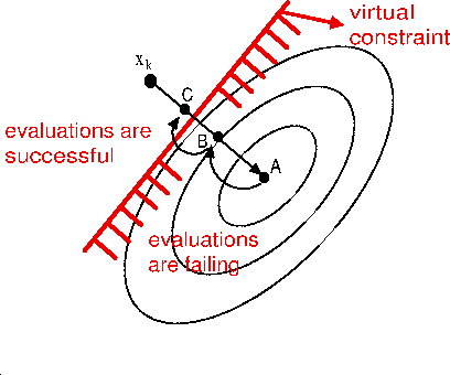
The simple strategy described above has strong limitations. In the example illustrated in figure 4.7, Condor will find as optimal solution the point A. If the same constraint is specified using a box or a linear constraint, Condor will be able to "slide" along it and to find the real optimum point, the point B.
In some cases you obtain as a result of an evaluation of the objective function
not only the value of the objective function itself but also the value of a
constraint which must be respected. For such constraint (which is linked to
the evaluation of the objective function), the strategy to use is the following:
use a penalty function.
What's a penalty function? Suppose you want to find:
Let's assume that you have a small violation of the constraints. In this case,
the equation 4.9 will directly penalizes
strongly the objective function. Equation 4.9
should be used if you don't want any violation at all at the end, optimal point
found by Condor. This is an advantage if equation 4.9.
A disadvantage appears when you choose too high values for ![]() and
and ![]() . This will produce strong non-linearities in the derivatives
of the new objective function 4.9 in the
part of the search space which is along the constraint (this is known as the
Maratos Effect). This will lead to a longer running time for the optimizer.
For some extreme values of
. This will produce strong non-linearities in the derivatives
of the new objective function 4.9 in the
part of the search space which is along the constraint (this is known as the
Maratos Effect). This will lead to a longer running time for the optimizer.
For some extreme values of ![]() and
and ![]() the optimizer can fail to find the optimum point of the objective
function.
the optimizer can fail to find the optimum point of the objective
function.
In opposition, the equation 4.10 does
not produce any non-linearity in the derivative, even for high values of ![]() and
and ![]() . This will lead to a short running time for the optimizer. However,
small violations of the constraints could be obtained at the end of the optimization
process.
. This will lead to a short running time for the optimizer. However,
small violations of the constraints could be obtained at the end of the optimization
process.
When using penalty functions, Condor can enter during the optimization process
in the infeasible space. However, if appropriate values are given to ![]() and
and ![]() , the optimal point found by Condor will be feasible (or, at least,
nearly feasible, when using equation 4.10
).
, the optimal point found by Condor will be feasible (or, at least,
nearly feasible, when using equation 4.10
).
You can easily define any penalty function inside Condor. All you have to do is to define a subAggregationFunction for each constraints. For example:
        <aggregationFunction>
              <subAggregationFunction name="main_function">
                 ... computation of f(x) ...
              </subAggregationFunction>
              <subAggregationFunction name="constraint_1">
               100 *  ... computation of c_1(x) ...
              </subAggregationFunction>
              <subAggregationFunction name="constraint_2">
               50 *  ... computation of c_2(x) ...
              </subAggregationFunction>
        </aggregationFunction>
In this example,
The extension to multiple linked-constraints is straight forward.
When possible, penalty functions should be avoid. In particular, if you have
simple box, linear or non-linear constraints, you should encode them inside
the XML file as standard constraints. Condor is using advanced techniques that
are (a lot) faster and are more robust in these cases.
Let's assume that you have an objective function that is computing some efficiency
measure (
![]() that you want to maximize. You will have something
like:
that you want to maximize. You will have something
like:
    <varNames dimension="2">
        x1 x2
    </varNames>
    <objectiveFunction nIndex="1">
        <indexNames> Efficiency </indexNames>
        <aggregationFunction>
              <subAggregationFunction name="good_main_function">
                -1.0 * Efficiency
              </subAggregationFunction>
              ... linked-constrained if any ...
        </aggregationFunction>
        <executableFile>
              ComputeEfficiency.exe
        </executableFile>
        ...
    </objectiveFunction>
You will never define:
        ...
        <aggregationFunction>
              <subAggregationFunction name="bad_main_function">
                (Efficiency-1)^2
              </subAggregationFunction>
              ...
Let's assume that the objective function
In future extension of the optimizer, the variables ![]() and
and ![]() will be adjusted automatically.
will be adjusted automatically.
Some optimizers which are working with constraints sometimes require to evaluate
the objective function in the infeasible space. This is for example the case
for the dual-simplex algorithm encountered in linear programming where all the
evaluations are in the infeasible space and only the last point of the optimization
process (the optimum point) is feasible.
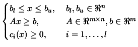
Condor is a 99% feasible optimizer. It means that 99% of the evaluations are
feasible. Basically, the Condor algorithm moves a cloud of points in the search
space towards the optimum point. The center of this cloud is ![]() and is always feasible. See illustration in figure 4.8.
The other points (the sampling point) are used to build (using Lagrange interpolation
technique)
and is always feasible. See illustration in figure 4.8.
The other points (the sampling point) are used to build (using Lagrange interpolation
technique)
![]()
![]() , the local approximation of the objective function
, the local approximation of the objective function ![]() around
around ![]() . These last points can be in the infeasible space. They are separated
from the center point
. These last points can be in the infeasible space. They are separated
from the center point ![]() (which is feasible) by a distance which is at most
(which is feasible) by a distance which is at most ![]() (see section 1.2 for
a complete explanation of these variables). Thus, the length of the violation
is at most
(see section 1.2 for
a complete explanation of these variables). Thus, the length of the violation
is at most ![]() .
.
You can see in figure 4.8
an illustration of these concepts. The green point is ![]() , the center of the cloud, the best point found so far. The blue
and red points are sampling points used to build
, the center of the cloud, the best point found so far. The blue
and red points are sampling points used to build
![]()
![]() . Some of these sampling points (the red ones) are in the infeasible
space. The length of the violation is at most
. Some of these sampling points (the red ones) are in the infeasible
space. The length of the violation is at most ![]() .
.
The external code which computes the objective function should always try
to give a correct evaluation of the objective function, even when an evaluation
is performed in the infeasible space. It should report a failure (see section
4.5 about failure in computation
of the objective function) in the least number of cases.
when using a penalty function (see section 4.6),
Condor can enter deeply into the infeasible space. However, at the end of the
optimization process, Condor will report the optimal feasible point (only for
appropriate values of ![]() and
and ![]() : see section 4.6
to know more about these variables).
: see section 4.6
to know more about these variables).