Noisy optimization

We will assume that objective functions derived from CFD codes have usually a simple shape but are subject to high-frequency, low amplitude noise. This noise prevents us to use simple finite-differences gradient-based algorithms. Finite-difference is highly sensitive to the noise. Simple Finite-difference quasi-Newton algorithms behave so badly because of the noise, that most researchers choose to use optimization techniques based on GA,NN,... [CAVDB01,PVdB98,Pol00]. The poor performances of finite-differences gradient-based algorithms are either due to the difficulty in choosing finite-difference step sizes for such a rough function, or the often cited tendency of derivative-based methods to converge to a local optimum [BDF$^+$98]. Gradient-based algorithms can still be applied but a clever way to retrieve the derivative information must be used. One such algorithm is DIRECT [GK95,Kel99,BK97] which is using a technique called implicit filtering. This algorithm makes the same assumption about the noise (low amplitude, high frequency) and has been successful in many cases [BK97,CGP$^+$01,SBT$^+$92]. For example, this optimizer has been used to optimize the cost of fuel and/or electric power for the compressor stations in a gas pipeline network [CGP$^+$01]. This is a two-design-variables optimization problem. You can see in the right of Figure 7.5 a plot of the objective function. Notice the simple shape of the objective function and the small amplitude, high frequency noise. Another family of optimizers is based on interpolation techniques. DFO, UOBYQA and CONDOR belongs to this last family. DFO has been used to optimize (minimize) a measure of the vibration of a helicopter rotor blade [BDF$^+$98]. This problem is part of the Boeing problems set [BCD$^+$95]. The blade are characterized by 31 design variables. CONDOR will soon be used in industry on a daily basis to optimize the shape of the blade of a centrifugal impeller [PMM$^+$03]. All these problems (gas pipeline, rotor blade and impeller blade) have an objective function based on CFD code and are both solved using gradient-based techniques. In particular, on the rotor blade design, a comparative study between DFO and other approaches like GA, NN,... has demonstrated the clear superiority of gradient-based techniques approach combined with interpolation techniques [BDF$^+$98].

We will now illustrate the performances of CONDOR in two simple cases which have sensibly the same characteristics as the objective functions encountered in optimization based on CFD codes. The functions, the amplitude of the artificial noise applied to the objective functions (uniform noise distribution) and all the parameters of the tests are summarized in Table 7.4. In this table ``NFE'' stands for Number of Function Evaluations. Each columns represents 50 runs of the optimizer.

Figure 7.3: Noisy optimization.

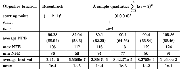Figure 7.4: On the left: A typical run for the optimization of the noisy Rosenbrock function. On the right:Four typical runs for the optimization of the simple noisy quadratic (noise=1e-4).

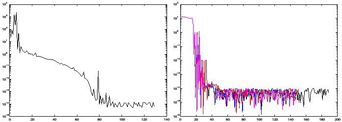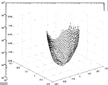
Figure 7.5: On the left: The relation between the noise (X axis) and the average best value found by the optimizer (Y axis). On the right: Typical shape of objective function derived from CFD analysis.

A typical run for the optimization of the noisy Rosenbrock function is given in the left of Figure 7.4. Four typical runs for the optimization of the simple noisy quadratic in four dimension are given in the right of figure 7.4. The noise on these four runs has an amplitude of 1e-4. In these conditions, CONDOR stops in average after 100 evaluations of the objective function but we can see in figure 7.4 that we usually already have found a quasi-optimum solution after only 45 evaluations.

As expected, there is a clear relationship between the noise applied on the objective function and the average best value found by the optimizer. This relationship is illustrated in the left of figure 7.4. From this figure and from the Table 7.4 we can see the following: When you have a noise of $10^{n+2}$, the difference between the best value of the objective function found by the optimizer AND the real value of the objective function at the optimum is around $10^{n}$. In other words, in our case, if you apply a noise of $10^{-2}$, you will get a final value of the objective function around $10^{-4}$. Obviously, this strange result only holds for this simple objective function (the simple quadratic) and these particular testing conditions. Nevertheless, the robustness against noise is impressive.

If this result can be generalized, it will have a great impact in the field of CFD shape optimization. This simply means that if you want a gain of magnitude $10^{n}$ in the value of the objective function, you have to compute your objective function with a precision of at least $10^{n+2}$. This gives you an estimate of the precision at which you have to calculate your objective function. Usually, the more precision, the longer the evaluations are running. We are always tempted to lower the precision to gain in time. If this strange result can be generalized, we will be able to adjust tightly the precision and we will thus gain a precious time.