| The optimum. We search for it. | |
 |
|
 |
|
|
|
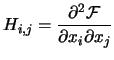
The Hessian Matrix of F at point |
|
|
The current approximation of the Hessian Matrix of F at point
If not stated explicitly, we will always assume |
|
|
The Hessian Matrix at the optimum point. |
|
|
|
|
|
|
|
|
|
|
|
|
|
|
| (2.1) |
| (2.2) |
| linear convergence |
|
| superlinear convergence |
|
| quadratic convergence |
|
 |
(2.3) |
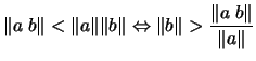
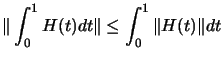 , and the cauchy-swartz inequality
 |
 with
with
![$\displaystyle \Vert g(v)-g(u) \Vert \geq \Bigg[ \frac{1}{\Vert H(x)^{-1} \Vert} -
\frac{\gamma}{2} (\Vert v-x\Vert+\Vert u-x\Vert) \Bigg] \Vert v-u\Vert $](img169.png)
![$\displaystyle \Vert g(v)-g(u) \Vert \geq \Bigg[ \frac{1}{\Vert H(x)^{-1} \Vert} - \gamma
\epsilon \Bigg] \Vert v-u\Vert $](img171.png)
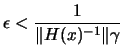 the lemma is proven with
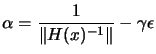 .
.
| 0 | |||
| 0 | |||
 |
 |
| 0 |  |
||
 |
(2.12) |
 . This implies that:
| (2.13) |
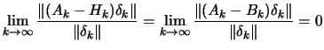 |
(2.14) |
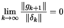
![\begin{figure}
\centering\fbox{\hspace{0.2cm}\parbox[t][5.2cm][b]{15.7cm}{
...
...\Vert}{\Vert\delta_k\Vert}=0\end{equation}} } }
\vspace{-0.1cm}
\end{figure}](img141.png)
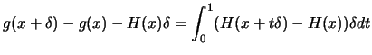
![\fbox{\hspace{0.2cm}\parbox[t][1.7cm][b]{15.7cm}{
{\em We will prove that if ...
...\Vert
( \Vert v-x\Vert + \Vert u-x\Vert )
\end{equation}\vspace{-.5cm} }
} }](img145.png)
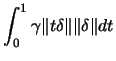
![\fbox{\hspace{0.2cm}\parbox[t][2.7cm][b]{15.7cm}{
{\em If $H$\ is Lipchitz co...
...hich
respect $ \max( \Vert v-x\Vert, \Vert u-x\Vert) \leq \epsilon$.\\ }
} }](img161.png)