Lazy Learning, Artificial Neural Networks and other functions approximators used inside a optimizer.

Figure 11.5: Lazy Learning identification

At the beginning of my research on continuous optimization, I was using the "Lazy Learning" as local model to guide the optimization process. Here is a brief resume of my unsuccessful experiences with the Lazy Learning.

Lazy learning is a local identification tool. Lazy learning postpones all the computation until an explicit request for a prediction is received. The request is fulfilled by modelling locally the relevant data stored in the database and using the newly constructed model to answer the request (see figure 11.5). Each prediction (or evaluation of the LL model) requires therefore a local modelling procedure. We will use, as regressor, a simple polynomial. Lazy Learning is a regression technique meaning that the newly constructed polynomial will NOT go exactly through all the points which have been selected to build the local model. The number of points used for the construction of this polynomial (in other words, the kernel size or the bandwidth) and the degree of the polynomial (0,1, or 2) are chosen using leave-one out cross-validation technique. The identification of the polynomial is performed using a recursive least square algorithm. The cross-validation is performed at high speed using PRESS statistics.

What is leave-one out cross-validation? This is a technique used to evaluate to quality of a regressor build on a dataset of $n$ points. First, take $n-1$ points from the dataset (These points are the training set). The last point $P$ will be used for validation purposes (validation set). Build the regressor using only the points in the training set. Use this new regressor to predict the value of the only point $P$ which has not been used during the building process. You obtain a fitting error between the true value of $P$ and the predicted one. Continue, in a similar way, to build regressors, each time on a different dataset of $n-1$ points. You obtain $n$ fitting errors for the $n$ regressors you have build. The global cross-validation error is the mean of all these $n$ fitting errors.

We will choose the polynomial which has the lowest cross-validation error and use it to answer the query.

We can also choose the $k$ polynomials which have the lowest cross-validation error and use, as final model, a new model which is the weighted average of these $k$ polynomials. The weight is the inverse of the leave-one out cross-validation error. In the Lazy learning toolbox, other possibilities of combination are possible.

When using artificial neural networks as local model, the number of neurons on the hidden layer is usually chosen using a leave-one out cross-validation ($loocv$) technique.

A simple idea is to use the leave-one out cross-validation error ($loocv$) to obtain an estimate of the quality of the prediction. An other simple idea is to use the $loocv$ to assess the validity of the model used to guide the optimization process. The validity of the local model is a very important notion. In CONDOR, the validity of the model is checked using equation 3.37 of chapter 3.4.2. No guarantee of convergence (even to a local optima) can be obtained without a local model which is valid.

When using Lazy Learning or Artificial Neural Networks as local models, we obtain the $loocv$, as a by-product of the computation of the approximator. Most of the time this $loocv$ is used to assess the quality of the approximator. I will now give a small example which demonstrate that the $loocv$ cannot be used to check the validity of the model. This will therefore demonstrate that Lazy Learning and Artificial Neural Networks cannot be used as local model to correctly guide the optimization process. Lazy Learning or Neural Networks can still be used but an external algorithm (not based on $loocv$) assessing their validity must be added (this algorithm is, most of the time, absent).

Figure 11.6: $loocv$ is useless to assess the quality of the model

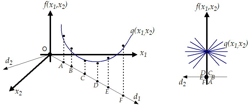
Let's consider the identification problem illustrated in figure 11.6. The local model $q(x_1,x2)$ of the function $f(x_1,x_2)$ to identify is build using the set of (points,values): $\{ (A,f(A)) ;$ $(B,f(B)) ;$ $(C,f(C)) ;$ $(D,f(D)) ;$ $(E,f(E)) ;$ $(F,f(F)) \}$. All these points are on the line $d_1$. You can see on the left of figure 11.6 that the leave-one out cross-validation error is very low: the approximator intercepts nearly perfectly the dataset. However there lacks some information about the function $f(x_1,x_2)$ to identify: In the direction $d_2$ (which is perpendicular to $d_1$) we have no information about $f(x_1,x_2)$. This leads to a simple infinity of approximators $q(x_1,x_2)$ which are all of equivalent (poor) quality. This infinity of approximators is illustrated on the right of figure 11.6. Clearly the model $q(x_1,x_2)$ cannot represents accurately $f(x_1,x_2)$. $q(x_1,x_2)$ is thus invalid. This is in contradiction with the low value of the $loocv$. Thus, the $loocv$ cannot be used to assess the quality of the model.

The identification dataset is composed of evaluation of $f(x)$ which are performed during the optimization process. Let's consider an optimizer based on line-search technique (CONDOR is based on trust region technique and is thus more robust). The algorithm is the following:

1. Search for a descent direction $s_k$ around $x_k$ ($x_k$ is the current position).

2. In the direction $s_k$, search the length $\alpha_k$ of the step.

3. Make a step in this direction: $x_{k+1}=x_k+\delta_k$ (with $\delta_k=\alpha_k s_k$)

4. Increment $k$. Stop if $\alpha_k \approx 0$ otherwise, go to step 1.

In the step 2 of this algorithm, many evaluation of $f(x)$ are performed aligned on the same line $s_k$. This means that the local,reduced dataset which will be used inside the lazy learning algorithm will very often be composed by aligned points. This situation is bad, as described at the beginning of this section. This explains why the Lazy Learning performs so poorly when used as local model inside a line-search optimizer. The situation is even worse than expected: the algorithm used inside the lazy learning to select the kernel size prevents to use points which are not aligned with $d_1$, leading to a poor, unstable model (complete explanation of this algorithm goes beyond the scope of this section). This phenomenon is well-known by statisticians and is referenced in the literature as "degeneration due to multi-collinearity" [Meyers1990]. The Lazy learning has actually no algorithm to prevent this degeneration and is thus of no-use in most cases.

To summarize: The validity of the local model must be checked to guarantee convergence to a local optimum. The leave-one out cross-validation error cannot be used to check the validity of the model. The lazy learning algorithm makes an extend use of the $loocv$ and is thus to proscribe. Optimizer which are using as local model Neural Networks, Fuzzy sets, or other approximators can still be used if they follow closely the surrogate approach [KLT97,BDF$^+$99] which is an exact and good method. In particular approach based on kriging models seems to give good results [BDF$^+$98].