The Lagrange Interpolation inside the optimization loop.

Inside the optimization program, we only use polynomials of degree lower or equal to 2. Therefore, we will always assume in the end of this chapter that $d=2$. We have thus $N=r_n^2=(n+1)(n+2)/2$ : the maximum number of monomials inside all the polynomials of the optimization loop.

A bound on the interpolation error.

We assume in this section that the objective function $f(x), x \in \Re^n$, has its third derivatives that are bounded and continuous. Therefore, if $y$ is any point int $\Re^n$, and if $\bar{d}$ is any vector int $\Re^n$ that has $\Vert \bar{d} \Vert=1$, then the function of one variable

$$\phi(\alpha)= f(y+\alpha \bar{d}), \quad \alpha \in \Re,$$ (3.26)

also has bounded and continuous third derivatives. Further there is a least non-negative number $M$, independent of $y$ and $\bar{d}$, such that every functions of this form have the property

$$\vert \phi'''(\alpha) \vert \leq M, \quad \alpha \in \Re$$ (3.27)

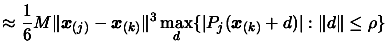
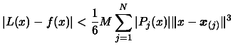
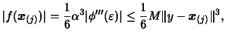
This value of M is suitable for the following bound on the interpolation error of f(x):

$$\vert L(x)-f(x) \vert < \frac{1}{6} M \sum_{j=1}^N \vert P_j(x) \vert \Vert x - \boldsymbol{x}_{(j)} \Vert^3$$ (3.28)

Proof
We make any choice of $y$. We regard $y$ as fixed for the moment, and we derive a bound on $\vert L(y)-f(y) \vert$. The Taylor series expansion of $f(x)$ around the point $y$ is important. Specifically, we let $T(x), x \in \Re^n$, be the quadratic polynomial that contains all the zero order, first order and second order terms of this expansion, and we consider the possibility of replacing the objective function $f$ by $f-T$. The replacement would preserve all the third derivatives of the objective function, because $T$ is a quadratic polynomial. Therefore, the given choice of M would remain valid. Further more, the quadratic model $f-T$ that is defined by the interpolation method would be $L-T$. It follows that the error on the new quadratic model of the new objective function is $f-L$ as before. Therefore, when seeking for a bound on $\vert L(y)-f(y) \vert$ in terms of third derivatives of the objective function, we can assume without loss of generality, that the function value $f(y)$, the gradient vector $g(y)=f'(y)$ and the second derivative matrix $H(y)=f''(y)$ are all zero.
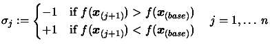
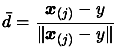
Let $j$ be an integer from $1, \ldots,N$ such that $\boldsymbol{x}_{(j)} \neq y$, let $\bar{d}$ be the vector:

$$\bar{d}= \frac{\boldsymbol{x}_{(j)}-y}{\Vert \boldsymbol{x}_{(j)}-y \Vert}$$ (3.29)

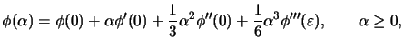
and let $\phi(\alpha), \alpha \in \Re$, be the function 3.28. The Taylor series with explicit remainder formula gives:

$$\phi(\alpha) = \phi(0) + \alpha \phi'(0) + \frac{1}{3} \alpha^2 \phi''(0) + \frac{1}{6} \alpha^3 \phi'''(\varepsilon), \quad \quad \alpha \geq 0,$$ (3.30)

where $\varepsilon$ depends on $\alpha$ and is in the interval $[0, \alpha]$. The values of $\phi(0)$, $\phi'(0)$ and $\phi''(0)$ are all zero due to the assumptions of the previous paragraph, and we pick $\alpha=\Vert y-\boldsymbol{x}_{(j)}\Vert$. Thus expressions 3.31, 3.28, 3.32, 3.29 provide the bound

$$\vert f(\boldsymbol{x}_{(j)}) \vert = \frac{1}{6} \alpha^3 \vert... ...'''(\varepsilon) \vert \leq \frac{1}{6} M \Vert y-\boldsymbol{x}_{(j)}\Vert^3,$$ (3.31)

which also holds without the middle part in the case $\boldsymbol{x}_{(j)}=y$, because of the assumption $f(y)=0$. Using $f(y)=0$ again, we deduce from Equation 3.26 and from inequality 3.33, that the error $L(y)-f(y)$ has the property:

$$\vert L(y)-f(y) \vert = \vert L(y) \vert = \vert \sum_{j=1}^N f(x_j) P_j(y) \vert$$

$$\leq \frac{1}{6} M \sum_{j=1}^N \vert P_j(y)\vert \Vert y-\boldsymbol{x}_{(j)}\Vert^3.$$

Therefore, because $y$ is arbitrary, the bound of equation 3.30 is true.
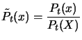
In the optimization loop, each time we evaluate the objective function f, at a point $x$, we adjust the value of an estimation of $M$ using:

$$M_{new}= \max \bigg[ M_{old}, \frac{\vert L(x)-f(x) \vert }{ \fr... ...sum_{j=1}^N \vert P_j(x) \vert \Vert x - \boldsymbol{x}_{(j)} \Vert^3 } \bigg]$$ (3.32)

Validity of the interpolation in a radius of $\rho$ around $\boldsymbol {x}_{(k)}$.

We will test the validity of the interpolation around $\boldsymbol {x}_{(k)}$. If the model (=the polynomial) is too bad around $\boldsymbol {x}_{(k)}$, we will replace the ``worst'' point $\boldsymbol{x}_{(j)}$ of the model by a new, better, point in order to improve the accuracy of the model.
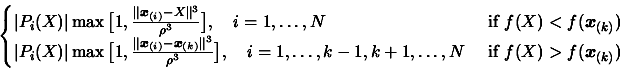
First, we must determine $x_j$. We select among the initial dataset $\{ \boldsymbol {x}_{(1)}, \ldots , \boldsymbol {x}_{(N)} \}$ a new dataset $\cal J$ which contains all the points $\boldsymbol{x}_{(i)}$ for which $\Vert \boldsymbol{x}_{(i)} - \boldsymbol{x}_{(k)} \Vert > 2 \rho$. If $\cal J$is empty, the model is valid and we exit.
We will check all the points inside $\cal J$, one by one.
We will begin by, hopefully, the worst point in $\cal J$: Among all the points in $\mbox{$\cal J$}$, choose the point the further away from $\boldsymbol {x}_{(k)}$. We define $j$ as the index of such a point.
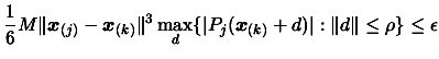
If $x$ is constrained by the trust region bound $\Vert x- \boldsymbol{x}_{(k)}\Vert < \rho$, then the contribution to the error of the model from the position $\boldsymbol{x}_{(j)}$ is approximately the quantity (using Equation 3.30):

$$\frac{1}{6}M \max_{x} \{ \vert P_j(x)\vert \Vert x- \boldsymbol{x}_{(k)} \Vert^3 : \Vert x- \boldsymbol{x}_{(k)} \Vert \leq \rho \}$$ (3.33)

$$\approx \frac{1}{6}M \Vert \boldsymbol{x}_{(j)}- \boldsymbol{x}_{... ...max_{d} \{ \vert P_j(\boldsymbol{x}_{(k)}+d)\vert : \Vert d \Vert \leq \rho \}$$ (3.34)

Therefore the model is considered valid if it satisfies the condition :

$$\frac{1}{6}M \Vert \boldsymbol{x}_{(j)}- \boldsymbol{x}_{(k)} \Ve... ...ert P_j(\boldsymbol{x}_{(k)}+d)\vert : \Vert d \Vert \leq \rho \} \leq \epsilon$$ (3.35)

$\epsilon$ is a bound on the error which must be given to the procedure which checks the validity of the interpolation. See section 6.1 to know how to compute the bound $\epsilon$.
The algorithm which searches for the value of $d$ for which we have

$$\max_{d} \{ \vert P_j(\boldsymbol{x}_{(k)}+d)\vert : \Vert d \Vert \leq \rho \}$$ (3.36)

is described in Chapter 5.
We are ignoring the dependence of the other Newton polynomials in the hope of finding a useful technique which can be implemented cheaply.
If Equation 3.37 is verified, we now remove the point $\boldsymbol{x}_{(j)}$ from the dataset $\mbox{$\cal J$}$ and we iterate: we search among all the points left in $\cal J$, for the point the further away from $\boldsymbol {x}_{(k)}$. We test this point using 3.37 and continue until the dataset $\mbox{$\cal J$}$ is empty.
If the test 3.37 fails for a point $\boldsymbol{x}_{(j)}$, then we change the polynomial: we remove the point $\boldsymbol{x}_{(j)}$ from the interpolating set and replace it with the ``better'' point: $\boldsymbol{x}_{(k)}+d$ (were $d$ is the solution of 3.38): see section 3.4.4, to know how to do.

Find a good point to replace in the interpolation.

If we are forced to include a new point $X$ in the interpolation set even if the polynomial is valid, we must choose carefully which point $\boldsymbol {x}_{(t)}$ we will drop.
Let us define $\boldsymbol {x}_{(k)}$, the best (lowest) point of the interpolating set.
We want to replace the point $\boldsymbol {x}_{(t)}$ by the point $X$. Following the remark of Equation 3.24, we must have:

$$\vert P_t(X) \vert \;$$ (3.37)

We also wish to remove a point which seems to be making a relatively large contribution to the bound 3.30 on the error on the quadratic model. Both of these objectives are observed by setting $t$ to the value of $i$ that maximizes the expression:

$$\begin{cases}\vert P_i(X)\vert \max \big[ 1, \frac{ \Vert \b... ...dots, N & \text{ if } f(X)>f(\boldsymbol{x}_{(k)}) \end{cases}$$ (3.38)

Replace the interpolation point $\boldsymbol {x}_{(t)}$ by a new point $X$.

Let $\tilde{P_i} \quad i=1,\ldots,N$, be the new Lagrange polynomials after the replacement of $\boldsymbol {x}_{(t)}$ by $X$.
The difference $\tilde{P_i}-P_i$ has to be a multiple of $\tilde{P_t}$, in order that $\tilde{P_i}$ agrees with $P_i$ at all the old interpolation points that are retained. Thus we deduce the formula:

$$\tilde{P_t}(x)= \frac{P_t(x)}{P_t(X)}$$ (3.39)

$$\tilde{P_i}(x)= P_i(x)- P_i(X) \tilde{P_t}(x), \quad i \neq t$$ (3.40)

$$L(x)=\sum_{j=1}^N f(\boldsymbol{x}_{(j)}) P_j(x)$$ has to be revised too. The difference $L_{new}-L_{old}$ is a multiple of $\tilde{P_t}(x)$ to allow the old interpolation points to be retained. We finally obtain:

$$L_{new}(x)=L_{old}(x)+ [ f(X) - L_{old}(X) ] \tilde{P_t}(x)$$ (3.41)

Generation of the first set of point $\{ \boldsymbol {x}_{(1)}, \ldots , \boldsymbol {x}_{(N)} \}$.

To be able to generate the first set of interpolation point $\{ \boldsymbol {x}_{(1)}, \ldots , \boldsymbol {x}_{(N)} \}$, we need:

• The base point $x_{(base)}$ around which $$\left\{ \begin{array}{l} \text{the function will be interpolated.} \\ \text{the set will be constructed} \end{array} \right.$$
• A length $\rho$ which will be used to separate 2 interpolation point.

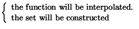
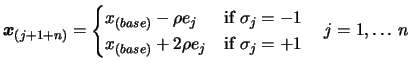
If we have already at disposal, $N=(n+1)(n+2)/2$ points situated inside a circle of radius $2 \; \rho$ around $x_{(base)}$, we try to construct directly a Lagrange polynomial using them. If the construction fails (points are not poised.), or if we don't have enough point we generate the following interpolation set:

• First point: $\boldsymbol{x}_{(1)}=x_{(base)}$
• From $\boldsymbol{x}_{(2)}$ to $\boldsymbol{x}_{(1+n)}$:
  $$\boldsymbol{x}_{(j+1)}=x_{(base)}+ \rho e_j \quad j=1, \ldots\, n \;$$    (with $e_i$ being a unit vector along the axis $j$ of the space)
  Let us define $\sigma_j$:
  $$\sigma_j := \begin{cases}-1 & \text{if } f(\boldsymbol{x}_{(j+1)}... ...ol{x}_{(j+1)}) < f(\boldsymbol{x}_{(base)}) \end{cases} \quad j=1, \ldots\, n$$

• From $\boldsymbol{x}_{(2+n)}$ to $\boldsymbol{x}_{(1+2n)}$:
  $$\boldsymbol{x}_{(j+1+n)}= \begin{cases}x_{(base)}- \rho e_j & \te... ...base)}+ 2 \rho e_j & \text{if } \sigma_j=+1 \end{cases} \quad j=1, \ldots\, n$$

• From $\boldsymbol{x}_{(2+2n)}$ to $\boldsymbol{x}_{(N)}$:
  Set $k=2+2n$.
  
  For $j=1, \ldots, n$
  
  1. For $i=1, \ldots, j-1$
     1. $$\boldsymbol{x}_{(k)} = x_{(base)}+ \rho ( \sigma_i e_i + \sigma_j e_j ) \quad 1\leq i<j\leq n$$
     2. Increment $k$.

Translation of a polynomial.

The precision of a polynomial interpolation is better when all the interpolation points are close to the center of the space ( $\Vert \boldsymbol{x}_{(i)} \Vert$ are small).
Example: Let all the interpolation points $\boldsymbol{x}_{(i)}$, be near $x_{(base)}$, and $\Vert x_{(base)}\Vert>>0$. We have constructed two polynomials $P_1(x)$ and $P_2(x)$:

• $P_1(x)$ interpolates the function $f(x)$ at all the interpolation sites $\boldsymbol{x}_{(i)}$.
• $P_2(x-x_{(base)})$ interpolates also the function $f(x)$ at all the interpolation sites $\boldsymbol{x}_{(i)}$.

$P_1(x)$ and $P_2(x)$ are both valid interpolator of $f(x)$ around $x_{(base)}$ BUT it's more interesting to work with $P_2$ rather then $P_1$ because of the greater accuracy in the interpolation.
How to obtain $P_2(x)$ from $P_1(x)$ ?
$P_2(x)$ is the polynomial $P_1(x)$ after the translation $x_{(base)}$.
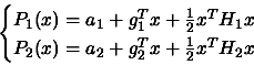
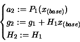
We will only treat the case where $P_1(x)$ and $P_2(x)$ are quadratics. Let's define $P1(x)$ and $P_2(x)$ the following way:

$$\begin{cases}P_1(x)= a_1 + g_1^T x + \frac{1}{2} x^T H_1 x \\ P_2(x)= a_2 + g_2^T x + \frac{1}{2} x^T H_2 x \end{cases}$$

Using the secant Equation 13.27, we can write:

$$\begin{cases}a_2 := P_1( x_{(base)} ) \\ g_2 := g_1 + H_1 x_{(base)} \\ H_2 := H_1 \end{cases}$$ (3.42)