Line-Search addenda.

Speed of convergence of Newton's method.

We have:

$$B_k \delta_k=-g_k$$ (13.1)

The Taylor series of $g$ around $x_k$ is:

$$g(x_k+h) = g(x_k)+B_k h+ o ( \Vert h\Vert^2 )$$

$$\Longleftrightarrow g(x_k-h) = g(x_k)-B_k h+ o ( \Vert h\Vert^2 )$$ (13.2)

If we set in Equation 13.2 $h=h_k=x_k-x^*$, we obtain :

$$g(x_k+h_k)=g(x^*)=\underline{0=g(x_k)-B_k h_k+o ( \Vert h_k\Vert^2 )}$$

If we multiply the left and right side of the previous equation by $B_k^{-1}$, we obtain, using 13.1:

$$\begin{array}{lrcl} &0&=&-\delta_k -h_k+o ( \Vert h_k\Vert... ...leftrightarrow &h_{k+1}&=&o ( \Vert h_k\Vert^2 ) \end{array}$$

By using the definition of $o$:

$$\Vert h_{k+1}\Vert < c \Vert h_k\Vert^2$$

with $c>0$.
This is the definition of quadratic convergence. Newton's method has quadratic convergence speed.

Note

If the objective function is locally quadratic and if we have exactly $B_k=H$, then we will find the optimum in one iteration of the algorithm.
Unfortunately, we usually don't have $H$, but only an approximation $B_k$ of it. For example, if this approximation is constructed using several ``BFGS update'', it becomes close to the real value of the Hessian $H$ only after $n$ updates. It means we will have to wait at least $n$ iterations before going in ``one step'' to the optimum. In fact, the algorithm becomes ``only'' super-linearly convergent.

How to improve Newton's method : Zoutendijk Theorem.

We have seen that Newton's method is very fast (quadratic convergence) but has no global convergence property ($B_k$ can be negative definite). We must search for an alternative method which has global convergence property. One way to prove global convergence of a method is to use Zoutendijk theorem.
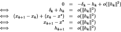
Let us define a general method:

1. find a search direction $s_k$
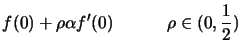
2. search for the minimum in this direction using 1D-search techniques and find $\alpha_k$ with

   $$x_{k+1}=x_k+\alpha_k s_k$$ (13.3)

   
   

3. Increment $k$. Stop if $g_k\approx 0$ otherwise, go to step 1.

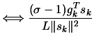
The 1D-search must respect the Wolf conditions. If we define $f(\alpha)=f(x+\alpha s)$, we have:

$$f(\alpha) \leq f(0) + \rho \alpha f'(0) \; \; \; \;\; \; \;\;\; \; \;\rho \in (0, \frac{1}{2})$$ (13.4)

$$f'(\alpha) > \sigma f'(0) \; \; \;\; \; \;\; \; \;\; \; \;\; \; \; \; \; \;\; \; \;\; \; \; \sigma \in (\rho,1)$$ (13.5)

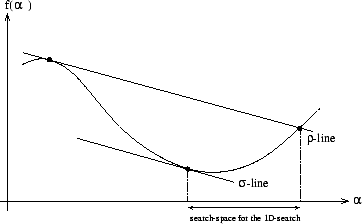
Figure 13.1: bounds on $\alpha$: Wolf conditions

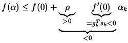
The objective of the Wolf conditions is to give a lower bound (equation 13.5) and upper bound (equation 13.4) on the value of $\alpha$, such that the 1D-search algorithm is easier: see Figure 13.1. Equation 13.4 expresses that the objective function $\mbox{$\cal F$}$ must be reduced sufficiently. Equation 13.5 prevents too small steps. The parameter $\sigma$ defines the precision of the 1D-line search:

• exact line search : $\sigma \approx 0.1$
• inexact line search : $\sigma \approx 0.9$
  

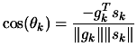
We must also define $\theta_k$ which is the angle between the steepest descent direction ($=-g_k$) and the current search direction ($=s_k$):

$$\cos(\theta_k)=\frac{-g_k^T s_k}{\Vert g_k \Vert \Vert s_k \Vert}$$ (13.6)

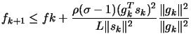
Under the following assumptions:

• $\mbox{$\cal F$}$$: \Re^n \rightarrow \Re$ bounded below
• $\mbox{$\cal F$}$ is continuously differentiable in a neighborhood $\cal N$ of the level set $\{ x \vert f(x) < f(x_1) \}$
• $g=\nabla f$ is lipschitz continuous:

  $$\exists L>0 : \; \Vert g(x)-g(\tilde{x}) \Vert < L \Vert x-\tilde{x} \Vert \; \; \; \forall x, \tilde{x} \in {\cal N}$$ (13.7)

  
  

We have:

$$\boldmath\sum_{k>1} \cos^2(\theta_k) \Vert g_k\Vert^2 < \infty$$ (13.8)

From Equation 13.5, we have:

$$f'(\alpha) > \sigma f'(0)$$

$$\Longleftrightarrow g_{k+1}^T s_k > \sigma g_k^T s_k$$

$$-g_k^T s_k$$

$$\Longleftrightarrow (g_{k+1}^T-g_k^T) s_k > (\sigma-1) g_k^T s_k$$ (13.9)

From Equation 13.7, we have:

$$\Vert g_{k+1}-g_k \Vert < L \Vert x_{k+1}-x_k \Vert$$ using Equation 13.3 :

$$\Longleftrightarrow \Vert g_{k+1}-g_k \Vert < \alpha_k L \Vert s_k \Vert$$

$$\Vert s_k \Vert$$

$$\Longleftrightarrow (g_{k+1}-g{k}^T) s_k <\Vert g_{k+1}-g_k \Vert \Vert s_k \Vert < \alpha_k L \Vert s_k \Vert^2$$ (13.10)

Combining Equation 13.9 and 13.10 we obtain:

$$(\sigma-1) g_k^T s_k < (g_{k+1}-g{k}^T) s_k < \alpha_k L \Vert s_k \Vert^2$$

$$\Longleftrightarrow \frac{(\sigma-1) g_k^T s_k}{L \Vert s_k \Vert^2} < \alpha_k$$ (13.11)

We can replace in Equation 13.4:

$$f(\alpha) \leq f(0) + \underbrace{\underbrace{\rho}_{>0} \; \; \; \; \underbrace{f'(0)}_{=g_k^T s_k<0}}_{<0} \alpha_k$$

the $\alpha_k$ by its lower bound from Equation 13.11. We obtain:

$$f_{k+1} \leq f{k}+\frac{\rho (\sigma-1) (g_k^T s_k)^2}{L \Vert s_k\Vert^2}\frac{ \Vert g_k\Vert^2}{\Vert g_k\Vert^2}$$

If we define $c=\frac{\rho (\sigma-1)}{L}<0$ and if we use the definition of $\theta_k$ (see eq. 13.6), we have:

$$f_{k+1} \leq f_k+ \underbrace{\underbrace{c}_{<0} \underbrace{\cos^2(\theta_k) \Vert g_k \Vert^2}_{>0}}_{<0}$$ (13.12)

$$\frac{f_{k+1}-f_k}{c} \geq \cos^2(\theta_k) \Vert g_k \Vert^2$$ (13.13)

Summing Equation 13.13 on k, we have

$$\frac{1}{c}\sum_k (f_{k+1}-f_k) \geq \sum_k\cos^2(\theta_k) \Vert g_k \Vert^2$$ (13.14)

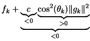
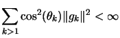
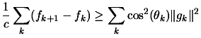
We know that $\mbox{$\cal F$}$ is bounded below, we also know from Equation 13.12, that $f_{k+1} \leq f_k$. So, for a given large value of k (and for all the values above), we will have $f_{k+1}=f_{k}$. The sum on the left side of Equation 13.14 converges and is finite: $\sum_k (f_{k+1}-f_k) < \infty$. Thus,we have:

$$\sum_{k>1} \cos^2(\theta_k) \Vert g_k\Vert^2 < \infty$$

which concludes the proof.

Angle test.

To make an algorithm globally convergent, we can make what is called an ``angle test''. It consists of always choosing a search direction such that $cos(\theta_k)> \epsilon >0$. This means that the search direction do not tends to be perpendicular to the gradient. Using the Zoutendijk theorem (see Equation 13.8), we obtain:

$$\lim_{k\rightarrow \infty} \Vert g_k \Vert = 0$$

which means that the algorithm is globally convergent.
The ``angle test'' on Newton's method prevents quadratical convergence. We must not use it.

The ``steepest descent'' trick.

If, regularly (lets say every $n+1$ iterations), we make a ``steepest descent'' step, we will have for this step, $cos(\theta_k)=1>0$. It will be impossible to have $cos(\theta_k)\rightarrow 0$. So, using Zoutendijk, the only possibility left is that $$\lim_{k\rightarrow \infty} \Vert g_k \Vert = 0$$. The algorithm is now globally convergent.