A simple direct optimizer: the Rosenbrock optimizer

The Rosenbrock method is a $0^{th}$ order search algorithm (i.e, it does not require any derivatives of the target function. Only simple evaluations of the objective function are used). Yet, it approximates a gradient search thus combining advantages of $0^{th}$ order and $1^{st}$ order strategies. It was published by Rosenbrock [Ros60] in the $70^{th}$.

This method is particularly well suited when the objective function does not require a great deal of computing power. In such a case, it's useless to use very complicated optimization algorithms. We will spend much time in the optimization calculations instead of making a little bit more evaluations of the objective function which will finally lead to a shorter calculation time.

Figure 13.5: Illustration of the Rosenbrock procedure using discrete steps (the number denotes the order in which the points are generated))

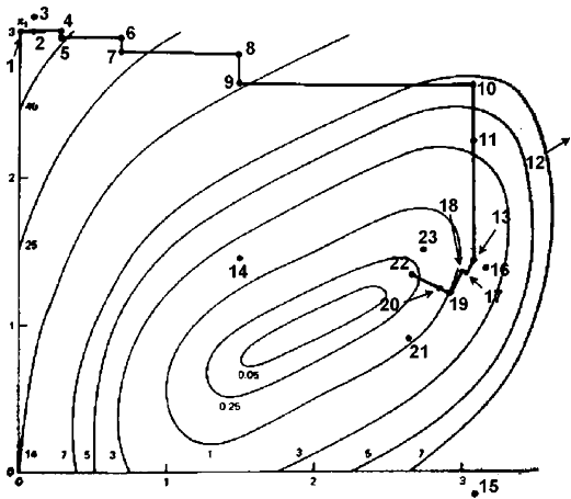In the first iteration, it is a simple $0^{th}$ order search in the directions of the base vectors of an n-dimensional coordinate system. In the case of a success, which is an attempt yielding a new minimum value of the target function, the step width is increased, while in the case of a failure it is decreased and the opposite direction will be tried (see points 1 to 15 in the Figure 13.5). Once a success has been found and exploited in each base direction, the coordinate system is rotated in order to make the first base vector point into the direction of the gradient (in Figure 13.5, the points 13, 16 & 17 are defining the new base). Now all step widths are initialized and the process is repeated using the rotated coordinate system (points 16 to 23).

The creation of a new rotated coordinate system is usually done using a Gram-Shmidt orthogonalization procedure. This algorithm is numerically instable. This instability can lead to a premature ending of the optimization algorithm. J.R.Palmer [Pal69] has proposed a beautiful solution to this problem.

Initializing the step widths to rather big values enables the strategy to leave local optima and to go on with search for more global minima. It has turned out that this simple approach is more stable than many sophisticated algorithms and it requires much less calculations of the target function than higher order strategies [Sch77]. This method has also been proved to always converge (global convergence to a local optima assured) [BSM93].

Finally a user who is not an optimization expert has a real chance to understand it and to set and tune its parameters properly.
The code of my implementation of the Rosenbrock algorithm is available in the code section. The code of the optimizer is standard C and doesn't use any special libraries. It can be compiled under windows or unix. The code has been highly optimized to be as fast as possible (with extend use of memcpy function, special fast matrix manipulation and so on...). The improvement of J.R. Palmer is used. This improvement allows still faster speed. The whole algorithm is only 107 lines long (with correct indentations). It's written in pure structural programmation (i.e., there is no ``goto instruction''). It is thus very easy to understand/customize. A small example of use (testR1.cpp) is available. In this example, the standard Rosenbrock banana function is minimized.