Levenberg-Marquardt algorithms
vs
Trust Region algorithms
Frank Vanden Berghen
IRIDIA, Université Libre de Bruxelles
50, av. Franklin Roosevelt
1050 Brussels, Belgium
Tel: +32 2 650 27 29, Fax: 32 2 650 27 15
For an in-depth explanation and more references about this subject, see my
thesis, section 2.1.
Let's assume that we want to find  , the minimum of the objective function

 .
.
Let us write the Taylor development limited to the degree 2 of
around  :
with
:
with
-

 , the quadratical approximation of
 around .
-
 , the gradient of
computed at .
, the gradient of
computed at .
-
 , an approximation of the real hessian matrix
  of
at .
of
at .
- , the real hessian matrix of
at .
For the moment, we will assume that  .
.
The unconstrained minimum  of
of
 is:
is:
Equation 1 is called the equation of the
Newton Step .
So, the Newton's method to find the minimum of
is:
- Set
 . Set
. Set
 .
.
- solve
 (go to the minimum of the current quadratical approximation
of
).
(go to the minimum of the current quadratical approximation
of
).
- set
- Increment
 . Stop if
 otherwise, go to step 2.
Newton's method is VERY fast: when is close to (when we are near the optimum) this method has quadratical convergence
speed:
with
 . Unfortunately, it does NOT always converge to the minimum
of
. To have convergence, we need to be sure that is always positive definite, ie. that the curvature of
is always positive.
. Unfortunately, it does NOT always converge to the minimum
of
. To have convergence, we need to be sure that is always positive definite, ie. that the curvature of
is always positive.
PROOF: must be positive definite to have convergence.
We want the search direction to be a descent direction
 |
(2) |
Taking the value of  from (1) and putting it in (2),
we have:
from (1) and putting it in (2),
we have:
The Equation (3) says that must always be positive definite.
END OF PROOF.
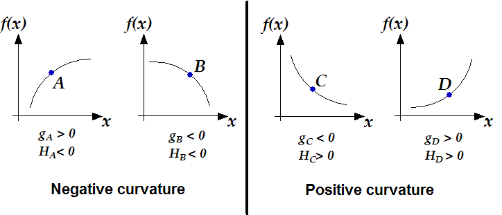
So, we must always construct the matrix so that it is a positive definite approximation of , the real Hessian matrix of
. The Newton's Algorithm cannot use negative curvature (when negative definite) inside
. . See figure 1 for an
illustration about positive/negative curvature.
Figure 1: positive/negative curvature of a function
 |
One possibility to solve this problem is to take  (
( =identity matrix), which is a very bad approximation of the Hessian
 but which is always positive definite. We will simply have
 . We will simply follow the slope. This algorithm is called
the ``steepest descent algorithm''. It is very slow. It has linear speed of convergence:
. We will simply follow the slope. This algorithm is called
the ``steepest descent algorithm''. It is very slow. It has linear speed of convergence:
 with
(problem is when
with
(problem is when
 ).
).
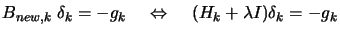
Another possibility, if we don't have positive definite, is to use instead
 with
with  being a very big number, such that
  is positive definite. Then we solve, as usual, the Newton
Step equation (see equation (1)):
is positive definite. Then we solve, as usual, the Newton
Step equation (see equation (1)):
 |
(4) |
Choosing a high value for has 2 effects:
- (inside equation
) will become negligible and we will find,
as search direction, ``the steepest descent step''.
- The step size
 is reduced.
In reality, only the above second point is important. It can be proven that, if
we impose a proper limitation on the step size
 , we maintain global convergence even if is an indefinite matrix. Trust region algorithms are based on this
principle (
, we maintain global convergence even if is an indefinite matrix. Trust region algorithms are based on this
principle ( is called the trust region radius). In trust region algorithm
the steps are:
is called the trust region radius). In trust region algorithm
the steps are:
 is the solution of is the solution of  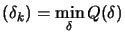 subject
to subject
to  |
(5) |
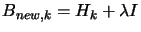
The old Levenberg-Marquardt algorithm uses a technique which adapts the value
of during the optimization. If the iteration was successful (
 ()), we decrease to exploit more the curvature information contained inside
. If the previous iteration was unsuccessful (
()), we decrease to exploit more the curvature information contained inside
. If the previous iteration was unsuccessful (
 ()), the quadratic model don't fit properly
the real function. We must then only use the ``basic'' gradient information. We
will increase in order to follow closely the gradient (``steepest descent
algorithm''). This old algorithm is the base for the explanation of the update
of the trust region radius in Trust Region Algorithms.
()), the quadratic model don't fit properly
the real function. We must then only use the ``basic'' gradient information. We
will increase in order to follow closely the gradient (``steepest descent
algorithm''). This old algorithm is the base for the explanation of the update
of the trust region radius in Trust Region Algorithms.
For intermediate value of , we will thus follow a direction which is a mixture of the
``steepest descent step'' and the ``Newton Step''. This direction is based on
a perturbated Hessian matrix and can sometime be disastrous (There is no geometrical meaning
of the perturbation  on ).
on ).
When a negative curvature is encountered ( negative definite):
- Newton's Method fail.
- Levenberg-Marquardt algorithms are following a perturbated and approximative
direction of research based on an arbitrary perturbation of ( is the solution of equation (4):
 ).
).
- Trust region algorithms will perform a long step (
 ) and ``move'' quickly to a more interesting
area (see equation (5))
) and ``move'' quickly to a more interesting
area (see equation (5))
Trust Region algorithm will thus exhibit better performances each time a negative
curvature is encountered and have thus better performances than all the Levenberg-Marquardt
algorithms. Unfortunately, the computation of for Trust Region algorithm involves a constrained minimization
of a quadratic subject to one non-linear constraint (see equation (5)).
This is not a trivial problem to solve at all. The algorithmic complexity of Trust
region algorithms is much higher. This explains why they are not very often encountered
despite their better performances. The solution of equation (5)
can be computed very efficiently using the fast algorithm from Moré and Sorensen.
There is one last point which must still be taken into account: How can we obtain
? Usually, we don't have the analytical expression of . must thus be approximated numerically. is usually constructed iteratively based on information gathered
from old evaluations
 for
for
 . Iterative construction of can be based on:
- The well-known BFGS formulae:
Each update is fast to compute but we get poor approximation of .
- Multivariate polynomial interpolation:
Each update is very time consuming. We get very precise .
- Finite difference approximation:
Very poor quality: numerical instability occurs very often.
To summarize:
- Levenberg-Marquardt algorithms and Trust region algorithms are both Newton
Step-based methods (they are called ``Restricted Newton Step methods''). Thus
they both exhibits quadratical speed of convergence near .
- When we are far from the solution ( far from ), we can encounter a negative curvature ( negative definite). If this happens, Levenberg-Marquardt algorithms
will slow down dramatically. In opposition, Trust Region Methods will perform
a very long step and ``move'' quickly to a more interesting area.
Old Levenberg-Marquardt algorithms were updating iteratively only on the iterations for which a good value for has been found (This is because on old computers the update
of is very time consuming, so we want to avoid it). Modern Levenberg-Marquardt
algorithms are updating iteratively at every iterations but they are still unable to follow a negative curvature inside the
function
. The steps remains thus of poor quality compared to trust region algorithms.
Levenberg-Marquardt algorithms are very often used to fit a non-linear function
through a set of points. Usually, to solve the fit, we will try to minimize the
sum of the squared intercept error (SOSE). In this case, the objective function
is convex and has always a positive curvature in all the point of the space. Levenberg-Marquardt
algorithms will thus have no problem and are usually well suited or these kinds
of problem.
To summarize: Trust Region Methods are an evolution of the Levenberg-Marquardt
algorithms. Trust Region Methods are able to follow the negative curvature of
the objective function. Levenberg-Marquardt algorithms are NOT able to do so and
are thus slower.