A small reminder about univariate interpolation.

We want to interpolate a simple curve $y=f(x), x \in \Re$ in the plane (in $\Re^2$). We have a set of $N$ interpolation points $(\boldsymbol{x}_{(i)}, f(\boldsymbol{x}_{(i)}) ), \quad i=1, \ldots, N \quad \boldsymbol{x}_{(i)} \in \Re$ on the curve. We can choose N as we want. We must have $\boldsymbol{x}_{(i)} \neq \boldsymbol{x}_{(j)}$ if $i \neq j$.

Lagrange interpolation

We define a Lagrange polynomial $P_i(x)$ as

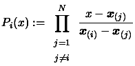$$P_i(x) := \prod_{ \begin{array}{c} \scriptstyle j=1 \\ \script... ... }^{N} \frac{x-\boldsymbol{x}_{(j)}}{\boldsymbol{x}_{(i)}-\boldsymbol{x}_{(j)}}$$ (3.2)

We will have the following property: 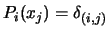$P_i(x_j)= \delta_{(i,j)}$ where $\delta_{(i,j)}$ is the Kronecker delta:

$$\delta_{(i,j)} = \begin{cases}0, & i \neq j; \\ 1, & i=j. \end{cases}$$ (3.3)

Then, the interpolating polynomial $L(x)$ is:

$$L(x)= \sum_{i=1}^N f(\boldsymbol{x}_{(i)}) \; P_i(x)$$ (3.4)

This way to construct an interpolating polynomial is not very effective because:

• The Lagrange polynomials $P_i(x)$ are all of degree $N$ and thus require lots of computing time for creation, evaluation and addition (during the computation of $L(x)$ )...
• We must know in advance all the $N$ points. An iterative procedure would be better.

The solution to these problems : The Newton interpolation.

Newton interpolation

The Newton algorithm is iterative. We use the polynomial $P_{k}(x)$ of degree $k-1$ which already interpolates $k$ points and transform it into a polynomial $P_{k+1}$ of degree $k$ which interpolates $k+1$ points of the function $f(x)$. We have:

$$P_{k+1}(x)= P_k(x)+ \quad ( x- \boldsymbol{x}_{(1)}) \cdots (x-\boldsymbol{x}_{(k)}) \quad [\boldsymbol{x}_{(1)}, \ldots, \boldsymbol{x}_{(k+1)}]f$$ (3.5)

The term $( x- \boldsymbol{x}_{(1)}) \cdots (x-\boldsymbol{x}_{(k)})$ assures that the second term of $P_{k+1}$ will vanish at all the points $\boldsymbol{x}_{(i)} \quad i=1, \ldots, k$.
Definition: $[\boldsymbol{x}_{(1)}, \ldots, \boldsymbol{x}_{(k+1)}]f$ is called a ''divided difference''. It's the unique leading coefficient (that is the coefficient of $x^k$) of the polynomial of degree $k$ that agree with $f$ at the sequence $\{ \boldsymbol{x}_{(1)}, \ldots, \boldsymbol{x}_{(k+1)} \}$.
The final Newton interpolating polynomial is thus:

$$P(x)= P_N(x) = \sum_{k=1}^N \quad ( x- \boldsymbol{x}_{(1)}) \cd... ...ymbol{x}_{(k-1)} ) \quad [\boldsymbol{x}_{(1)}, \ldots, \boldsymbol{x}_{(k)}]f$$ (3.6)

The final interpolation polynomial is the sum of polynomials of degree varying from 0 to $N-1$ (see Equation 3.5). The manipulation of the Newton polynomials (of Equation 3.5) is faster than the Lagrange polynomials (of Equation 3.2) and thus, is more efficient in term of computing time. Unfortunately, with Newton polynomials, we don't have the nice property that $P_i(x_j)= \delta_{(i,j)}$.
We can already write two basic properties of the divided difference:

$$[ \boldsymbol{x}_{(k)} ]f= f( \boldsymbol{x}_{(k)})$$ (3.7)

$$[ \boldsymbol{x}_{(1)}, \boldsymbol{x}_{(2)} ]f= \frac{f( \boldsy... ...(2)})- f( \boldsymbol{x}_{(1)})}{\boldsymbol{x}_{(2)} - \boldsymbol{x}_{(1)} }$$ (3.8)

The divided difference for the Newton form.

Lemma 1

We will proof this by induction. First, we rewrite Equation 3.9, for N=1, using 3.7:

$$f(x)= f(\boldsymbol{x}_{(1)}) + (x- \boldsymbol{x}_{(1)})[\boldsymbol{x}_{(1)}, x]f$$ (3.9)

Using Equation 3.8 inside 3.10, we obtain:

$$f(x)= f(\boldsymbol{x}_{(1)}) + (x- \boldsymbol{x}_{(1)}) \frac{ f( x )- f( \boldsymbol{x}_{(1)})}{x - \boldsymbol{x}_{(1)} }$$ (3.10)

This equation is readily verified. The case for $N=1$ is solved. Suppose the Equation 3.9 verified for $N=k$ and proof that it will also be true for $N=k+1$. First, let us rewrite equation 3.10, replacing $\boldsymbol{x}_{(1)}$ by $\boldsymbol{x}_{(k+1)}$ and replacing $f(x)$ by $[\boldsymbol{x}_{(1)}, \ldots, \boldsymbol{x}_{(k)}, x]f$ as a function of x. (In other word, we will interpolate the function $f(x) \equiv [\boldsymbol{x}_{(1)}, \ldots, \boldsymbol{x}_{(k)}, x]f$ at the point $\boldsymbol{x}_{(k+1)}$ using 3.10.) We obtain:

$$[\boldsymbol{x}_{(1)}, \ldots, \boldsymbol{x}_{(k)}, x]f = [\bol... ...,x] \bigg([\boldsymbol{x}_{(1)}, \ldots, \boldsymbol{x}_{(k)}, \cdot ]f \bigg)$$ (3.11)

Let us rewrite Equation 3.9 with $N=k$.

$$f(x)= P_k(x) + ( x- \boldsymbol{x}_{(1)}) \cdots (x-\boldsymbol{x}_{(k)} ) \quad [x_1, \ldots, x_k, x]f$$ (3.12)

Using Equation 3.12 inside Equation 3.13:

$$f(x)= P_{k+1}(x) + ( x- \boldsymbol{x}_{(1)}) \cdots (x-\boldsymb... ...,x] \bigg([\boldsymbol{x}_{(1)}, \ldots, \boldsymbol{x}_{(k)}, \cdot ]f \bigg)$$ (3.13)

Let us rewrite Equation 3.5 changing index $k+1$ to $k+2$.

$$P_{k+2}(x)= P_{k+1}(x)+ \quad ( x- \boldsymbol{x}_{(1)}) \cdots ... ...ymbol{x}_{(k+1)}) \quad [\boldsymbol{x}_{(1)}, \ldots, \boldsymbol{x}_{(k+2)}]f$$ (3.14)

Recalling the definition of the divided difference: $[x_1, \ldots, x_{k+2}]f$ is the unique leading coefficient of the polynomial of degree $k+1$ that agree with $f$ at the sequence $\{ \boldsymbol{x}_{(1)}, \ldots, \boldsymbol{x}_{(k+2)} \}$. Because of the uniqueness and comparing equation 3.14 and 3.15, we see that (replacing $x$ by $\boldsymbol{x}_{(k+2)}$ in 3.14):

$$[\boldsymbol{x}_{(k+1)},\boldsymbol{x}_{(k+2)}] \bigg([\boldsymb... ...k)}, \cdot ]f \bigg) = [\boldsymbol{x}_{(1)}, \ldots, \boldsymbol{x}_{(k+2)}]f$$ (3.15)

Using Equation 3.16 inside 3.14:

$$f(x)= P_{k+1}(x) + ( x- \boldsymbol{x}_{(1)}) \cdots (x-\boldsymbol{x}_{(k+1)} ) [\boldsymbol{x}_{(1)}, \ldots, \boldsymbol{x}_{(k+2)}]f$$ (3.16)

Recalling the discussion of the paragraph after Equation 3.11, we can say then this last equation complete the proof for $N=k+1$. The lemma 1 is now proved.
Lemma 2

This is clear from the definition of $[\boldsymbol{x}_{(1)}, \ldots, \boldsymbol{x}_{(k)}]f$.
Lemma 3

Combining Equation 3.16 and Equation 3.8, we obtain:

$$\frac{ [\boldsymbol{x}_{(1)}, \ldots, \boldsymbol{x}_{(k)}, \bold... ...\boldsymbol{x}_{(k+1)}}=[\boldsymbol{x}_{(1)}, \ldots, \boldsymbol{x}_{(k+2)}]f$$ (3.17)

Using Equation 3.19 and lemma 2, we obtain directly 3.18. The lemma is proved.
Equation 3.18 has suggested the name ``divided difference''.

$$\hspace{-1cm} \begin{array}{ccccccc} \text{interp.} & & \te... ...dsymbol{x}_{(N)} & f(\boldsymbol{x}_{(N)}) &&&&& \end{array}$$

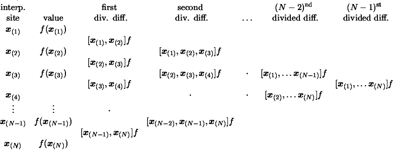
We can generate the entries of the divided difference table column by column from the given dataset using Equation 3.18. The top diagonal then contains the desired coefficients $[\boldsymbol{x}_{(1)}]f$ , $[\boldsymbol{x}_{(1)}, \boldsymbol{x}_{(2)}]f , [\boldsymbol{x}_{(1)}, \bolds... ...mbol{x}_{(3)}]f ,\ldots, [\boldsymbol{x}_{(1)}, \ldots, \boldsymbol{x}_{(N)}]f$ of the final Newton form of Equation 3.6.

The Horner scheme

Suppose we want to evaluate the following polynomial:

$$P(x)= c_0 + c_1 x + c_2 x^2 + c_3 x^3 + c_4 x^4$$ (3.18)

We will certainly NOT use the following algorithm:

1. Initialisation $r=c_0$
2. For $k=2, \ldots, N$
   1. Set $r:=r+ c_k x^k$
3. Return $r$

This algorithm is slow (lots of multiplications in $x^k$) and leads to poor precision in the result (due to rounding errors).
The Horner scheme uses the following representation of the polynomial 3.20: 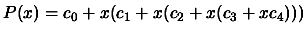$P(x)= c_0 + x ( c_1 + x ( c_2 + x ( c_3 + x c_4 )))$, to construct a very efficient evaluation algorithm:

1. Initialisation $r=c_N$
2. For $k=N-1, \ldots, 0$
   1. Set $r:=c_k+ x \; r$
3. Return $r$

There is only $N-1$ multiplication in this algorithm. It's thus very fast and accurate.