Next: Finding the root of
Up: The Trust-Region subproblem
Previous: must be positive definite.
Contents
Subsections
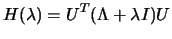
Theorem 2 tells us that we should be looking for solutions to
4.9 and implicitly tells us what value of  we
need. Suppose that
we
need. Suppose that  has an eigendecomposition:
 |
(4.8) |
where  is a diagonal matrix of eigenvalues
 and
and  is an
orthonormal matrix of associated eigenvectors. Then
is an
orthonormal matrix of associated eigenvectors. Then
 |
(4.9) |
We deduce immediately
from Theorem 2 that the value of we seek must satisfy
![$ \lambda^* > \min [ 0, -\lambda_1 ]$](img577.png) (as only then is
(as only then is
 positive semidefinite) (
 is the least eigenvalue of
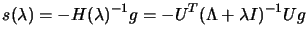
). We can compute a solution
is the least eigenvalue of
). We can compute a solution
 for a given value of
using:
for a given value of
using:
 |
(4.10) |
The solution we are looking for
depends on the non-linear inequality
 . To say more we need to examine
 in detail.
For convenience we define
in detail.
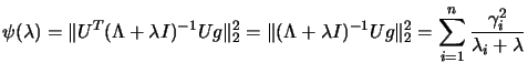
For convenience we define
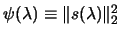 . We have that:
 |
(4.11) |
where
 is
is ![$ [Ug]_i$](img585.png) , the
, the  component of
  .
.
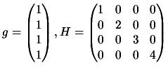
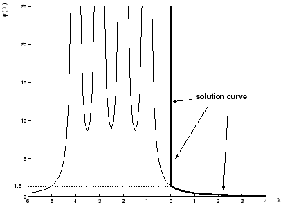
Suppose the problem is defined by:
We plot
the function
 in Figure 4.1. Note the
pole of
at the negatives of each eigenvalues of
. In view of theorem 2, we are only interested in
in Figure 4.1. Note the
pole of
at the negatives of each eigenvalues of
. In view of theorem 2, we are only interested in
 . If
. If  , the optimum lies inside the trust region
boundary. Looking at the figure, we obtain
, the optimum lies inside the trust region
boundary. Looking at the figure, we obtain
 ,
for
,
for
 . So, it means that if
 , we have an internal optimum which can be computed
using 4.9. If
, we have an internal optimum which can be computed
using 4.9. If
 , there is a unique value of
 (given in the figure and by
 |
(4.12) |
which, used inside
4.9, give the optimal  .
.
Figure 4.1:
A plot of
for positive
definite.
 |
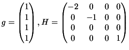
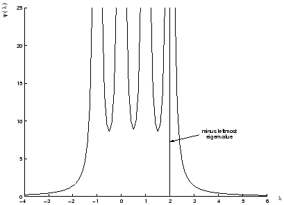
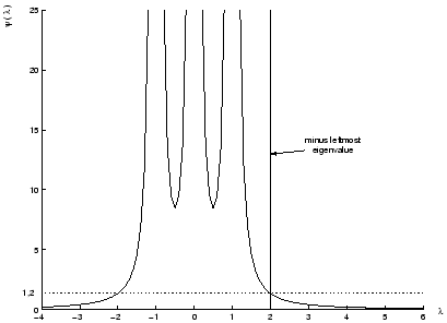
Suppose the problem is defined by:
We plot
the function
in Figure 4.2. Recall that
is defined as the least eigenvalue of . We are only
interested in values of
 , that is
 . For value of
 , we have
NOT
positive definite. This is forbidden due to theorem 2. We can see
that for any value of
, we have
NOT
positive definite. This is forbidden due to theorem 2. We can see
that for any value of  , there is a corresponding value of
. Geometrically, H is indefinite, so the model function
is unbounded from below. Thus the solution lies on the
trust-region boundary. For a given
, there is a corresponding value of
. Geometrically, H is indefinite, so the model function
is unbounded from below. Thus the solution lies on the
trust-region boundary. For a given  , found using
4.14, we obtain the optimal using 4.9.
, found using
4.14, we obtain the optimal using 4.9.
Figure 4.2:
A plot of
for
indefinite.
 |
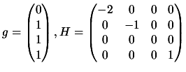
Suppose the problem is defined by:
We plot
the function
in Figure 4.3. Again,
 , is forbidden due to theorem 2. If,
 , there is no acceptable value of
. This difficulty can only arise when
, there is no acceptable value of
. This difficulty can only arise when  is orthogonal
to the space
is orthogonal
to the space  , of eigenvectors corresponding to the most
negative eigenvalue of . When
, of eigenvectors corresponding to the most
negative eigenvalue of . When
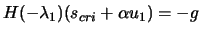
 , then
equation 4.9 has a limiting solution
, then
equation 4.9 has a limiting solution  , where
 .
.
Figure 4.3:
A plot of
for
semi-definite and singular(hard case).
 |
 is positive semi-definite and singular and
therefore 4.9 has several solutions. In particular, if
is positive semi-definite and singular and
therefore 4.9 has several solutions. In particular, if
 is an eigenvector corresponding to , we have
 , and thus:
 |
(4.13) |
holds for any value of the
scalar  . The value of can be chosen so that
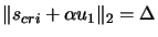 . There are two roots to this
equation:
. There are two roots to this
equation:  and
and  . We evaluate the model at
these two points and choose as solution
. We evaluate the model at
these two points and choose as solution
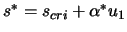 , the lowest one.
Next: Finding the root of
Up: The Trust-Region subproblem
Previous: must be positive definite.
Contents
Frank Vanden Berghen
2004-04-19