


Next: The secant equation
Up: Annexes
Previous: Gram-Schmidt orthogonalization procedure.
Contents
Notions of constrained optimization
Let us define the problem:
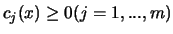
Find the minimum of  subject to
  constraints
 .
.
Figure 13.2:
Existence of Lagrange Multiplier 
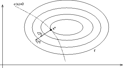 |
To be at an optimum point  we must have the equi-value line
(the contour) of tangent to the constraint border
we must have the equi-value line
(the contour) of tangent to the constraint border  .
In other words, when we have
.
In other words, when we have  constraints, we must have (see
illustration in Figure 13.2) (the gradient of
constraints, we must have (see
illustration in Figure 13.2) (the gradient of  and the gradient of
  must aligned):
In the more general case when
must aligned):
In the more general case when  , we have:
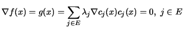 |
(13.19) |
Where E is the set of active constraints, that is, the constraints
which have  We define Lagrangian function
  as:
as:
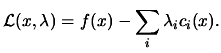 |
(13.20) |
The Equation 13.19 is then equivalent to:
![$\displaystyle \begin{picture}(.27,.3)
\put(0,0){\makebox(0,0)[bl]{$\nabla$}}
\put(.16,.17){\circle*{.18}} \end{picture}
\L (x^*,\lambda^*)=0$](img1379.png) where where ![$\displaystyle \begin{picture}(.27,.3)
\put(0,0){\makebox(0,0)[bl]{$\nabla$}}
...
...e}
= \left( \begin{array}{c}
\nabla_x \\ \nabla_\lambda
\end{array} \right)$](img1380.png) |
(13.21) |
In unconstrained optimization, we found an optimum when
 . In constrained optimization, we find an optimum point
(
. In constrained optimization, we find an optimum point
(
 ), called a KKT point (Karush-Kuhn-Tucker point)
when:
), called a KKT point (Karush-Kuhn-Tucker point)
when:
 is a KKT point is a KKT point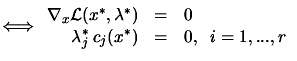 |
(13.22) |
Figure 13.3:
complementarity condition
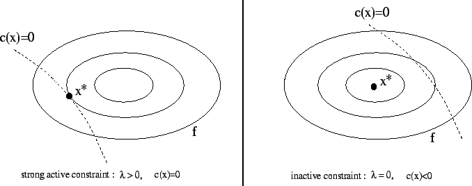 |
The second equation of 13.22 is called the
complementarity condition. It states that both  and
and
 cannot be non-zero, or equivalently that inactive
constraints have a zero multiplier. An illustration is given on
figure 13.3.
cannot be non-zero, or equivalently that inactive
constraints have a zero multiplier. An illustration is given on
figure 13.3.
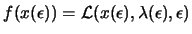
To get an other insight into the meaning of Lagrange Multipliers
, consider what happens if the right-hand sides of the
constraints are perturbated, so that
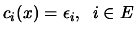 |
(13.23) |
Let
 ,
,
 denote how the solution and multipliers change
as
denote how the solution and multipliers change
as  changes. The Lagrangian for this problem is:
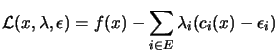 |
(13.24) |
From 13.23,
 , so
using the chain rule, we have
, so
using the chain rule, we have
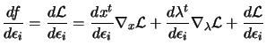 |
(13.25) |
Using Equation 13.21, we see that the
terms
 and
and
 are null in the
previous equation. It follows that:
are null in the
previous equation. It follows that:
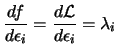 |
(13.26) |
Thus the Lagrange
multiplier of any constraint measure the rate of change in the
objective function, consequent upon changes in that constraint
function. This information can be valuable in that it indicates
how sensitive the objective function is to changes in the
different constraints.
Next: The secant equation
Up: Annexes
Previous: Gram-Schmidt orthogonalization procedure.
Contents
Frank Vanden Berghen
2004-04-19