Next: The Lagrange Interpolation inside
Up: Multivariate Lagrange Interpolation
Previous: A small reminder about
Contents
Subsections
We want to interpolate an hypersurface
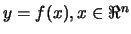 in
the dimension
in
the dimension  . We have a set of interpolation points
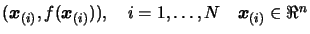 on the surface. We must be sure that the problem is
well poised: The number
on the surface. We must be sure that the problem is
well poised: The number  of points is
  and the
Vandermonde determinant is not null.
We will construct our polynomial basis
and the
Vandermonde determinant is not null.
We will construct our polynomial basis
 iteratively. Assuming that we already have a polynomial

 interpolating
  points, we
will add to it a new polynomial
points, we
will add to it a new polynomial  which doesn't destruct
all what we have already done. That is the value of
which doesn't destruct
all what we have already done. That is the value of
 must be zero for
 . In
other words,
. In
other words,
 . This is easily
done in the univariate case:
. This is easily
done in the univariate case:
 , but in the multivariate case, it becomes
difficult.
, but in the multivariate case, it becomes
difficult.
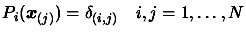
We must find a new polynomial which is somewhat
''perpendicular'' to the
 with respect to
the points
with respect to
the points
 . Any multiple of
added to the previous
. Any multiple of
added to the previous  must leave the value of this
unchanged at the points
.
We can see the polynomials as ``vectors'', we search for a
new ``vector'' which is ``perpendicular'' to all the
. We will use a version of the Gram-Schmidt othogonalisation
procedure adapted for the polynomials. The original Gram-Schmidt
procedure
for vectors is described in the annexes in Section 13.2.
must leave the value of this
unchanged at the points
.
We can see the polynomials as ``vectors'', we search for a
new ``vector'' which is ``perpendicular'' to all the
. We will use a version of the Gram-Schmidt othogonalisation
procedure adapted for the polynomials. The original Gram-Schmidt
procedure
for vectors is described in the annexes in Section 13.2.
We define the scalar product with respect to the dataset  of points
 between the two
polynomials
between the two
polynomials  and
and  to be:
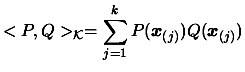 |
(3.19) |
We have a set of independent polynomials
 . We want to convert this set
into a set of orthonormal vectors
. We want to convert this set
into a set of orthonormal vectors
 with respect to the dataset of points
 by the Gram-Schmidt process:
- Initialization k=1;
- Normalisation
 |
(3.20) |
- Orthogonalisation
For  to ,
to ,  do:
do:
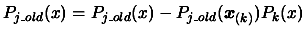 |
(3.21) |
We will take each
 and remove
from it the component parallel to the current polynomial
and remove
from it the component parallel to the current polynomial  .
.
- Loop increment . If
 go to step 2.
After completion of the algorithm, we discard all the
's and replace them with the  's for the next
iteration of the global optimization algorithm.
's for the next
iteration of the global optimization algorithm.
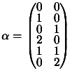
The initial set of polynomials
 can simply
by initialized with the monomials of a polynomial of dimension
can simply
by initialized with the monomials of a polynomial of dimension
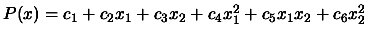
 . For example, if
  , we obtain:
  ,
,
 ,
,
 ,
,
 ,
,
 ,
,
 ,
,
 ,
,
 ,
, 
In the Equation 3.22, there is a division. To improve the
stability of the algorithm, we must do ``pivoting''. That is:
select a salubrious pivot element for the division in Equation
3.22). We should choose the
 (among the points
which are still left inside the dataset) so that the denominator
of Equation 3.22 is far from zero:
(among the points
which are still left inside the dataset) so that the denominator
of Equation 3.22 is far from zero:
 as great as possible. as great as possible. |
(3.22) |
If we don't
manage to find a point
 such that
 , it means the dataset is NOT poised and the algorithm fails.
After completion of the algorithm, we have:
 |
(3.23) |
The Lagrange interpolation polynomial  .
.
Using Equation 3.25, we can write:
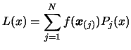 |
(3.24) |
Lets us rewrite a polynomial of degree  and dimension using
the following notation ():
and dimension using
the following notation ():
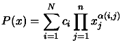 with with 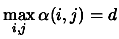 |
(3.25) |
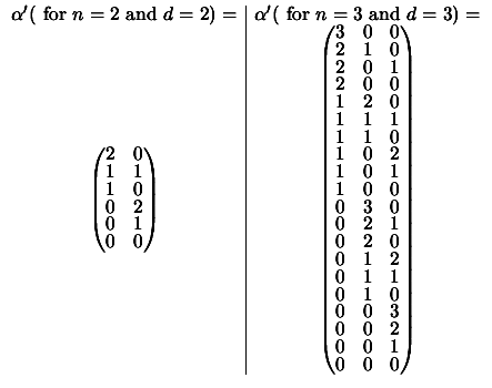
 is a matrix which represents the way the monomials are
ordered inside the polynomial. Inside our program, we always use
the ``order by degree'' type. For example, for
is a matrix which represents the way the monomials are
ordered inside the polynomial. Inside our program, we always use
the ``order by degree'' type. For example, for  , we
have:
, we
have:
 . We have the following matrix :
We can also use the ``inverse lexical order''. For example,
for , we have:
 . We have the following matrix
 (the
(the  is to indicate that we are in ``inverse lexical
order'') :
This matrix is constructed using the following property of the
''inverse lexical order'':
is to indicate that we are in ``inverse lexical
order'') :
This matrix is constructed using the following property of the
''inverse lexical order'':
and
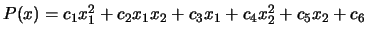
The ``inverse lexical order'' is easier to transform in a
multivariate horner scheme. For example: for the polynomial
 , we have:
- Set
- Set

- Set
- Set

- Set
- Return
You can see that we retrieve inside this decomposition of the algorithm for the
evaluation of the polynomial  , the coefficient
  in the same order that they appear when ordered in ``inverse lexical
order''.
in the same order that they appear when ordered in ``inverse lexical
order''.
Let us define the function
 . This function takes, as
input, the index of a monomial inside a polynomial ordered by
''inverse lexical order'' and gives, as output, the index of the
same monomial but, this time, placed inside a polynomial ordered
''by degree''. In other words, This function makes the
TRansformation between index in inverse lexical order and index
ordered by degree.
. This function takes, as
input, the index of a monomial inside a polynomial ordered by
''inverse lexical order'' and gives, as output, the index of the
same monomial but, this time, placed inside a polynomial ordered
''by degree''. In other words, This function makes the
TRansformation between index in inverse lexical order and index
ordered by degree.
We can now define an algorithm which computes the value of a
multivariate polynomial ordered by degree by multivariate horner
scheme:
- Declaration
: dimension of the space
 : number of monomial inside a polynomial of
dimension and degree .
: number of monomial inside a polynomial of
dimension and degree .
 : registers for summation (
 )
)
 : counters (
 )
)
 : the coefficients of the polynomial
ordered by degree.
: the coefficients of the polynomial
ordered by degree.
- Initialization
Set

set
- For

- Determine
- Set

- Set
- Set
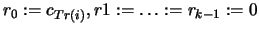
- Set
- Return
In the program, we are caching the values of k and the function
TR, for a given and . Thus, we compute these values once,
and use pre-computed values during the rest of the time. This lead
to a great efficiency in speed and in precision for polynomial
evaluations.
Next: The Lagrange Interpolation inside
Up: Multivariate Lagrange Interpolation
Previous: A small reminder about
Contents
Frank Vanden Berghen
2004-04-19