


Next: The bound .
Up: Unconstrained Optimization
Previous: About the choice of
Contents
The CONDOR unconstrained algorithm.
I strongly suggest the reader to read first the Section
2.4 which presents a global, simplified view of
the algorithm. Thereafter, I suggest to read this section,
disregarding the parallel extensions which are not useful to
understand the algorithm.
Let  be the dimension of the search space.
Let  be the objective function to minimize.
Let  be the starting point of the algorithm.
Let
 and
and
 be the initial and final value
of the global trust region radius.
be the initial and final value
of the global trust region radius.
Let  and
and  , be the absolute and relative errors
on the evaluation of the objective function.
, be the absolute and relative errors
on the evaluation of the objective function.
- Set
 ,
,
 and generate a first
interpolation set
and generate a first
interpolation set
 around
(with
around
(with
 ), using technique described in
section 3.4.5 and evaluate the objective function at
these points.
), using technique described in
section 3.4.5 and evaluate the objective function at
these points.
Parallel extension: do the  evaluations in parallel
in a cluster of computers
evaluations in parallel
in a cluster of computers
- Choose the index
 of the best (lowest) point of the set

 . Let
. Let
 . Set
. Set
 . Apply a translation of
 to all the dataset
and generate the polynomial
to all the dataset
and generate the polynomial  of degree 2, which
intercepts all the points in the dataset (using the technique
described in Section 3.3.2 ).
of degree 2, which
intercepts all the points in the dataset (using the technique
described in Section 3.3.2 ).
- Parallel extension: Start the parallel process: make a
local copy
 of and use it to choose good
sampling site using Equation 3.38 on
.
of and use it to choose good
sampling site using Equation 3.38 on
.
- Parallel extension: Check the results of the
computation made by the parallel process. Update using all
these evaluations. We will possibly have to update the index
of the best point in the dataset and
 . Replace
  with a fresh copy of .
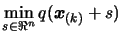
- Find the trust region step
 , the solution of
 subject to
 , using the technique described in Chapter
4.
, using the technique described in Chapter
4.
In the constrained case, the trust region step is the solution of:
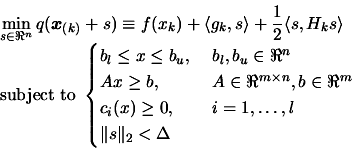 |
(6.1) |
where  are the box constraints,
  are the linear constraints and
 are the non-linear
constraints.
are the non-linear
constraints.
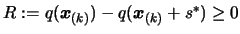
- If
 , then break and
go to step 16: we need to be sure that the model is valid before
doing a step so small.
, then break and
go to step 16: we need to be sure that the model is valid before
doing a step so small.
- Let
 , the predicted
reduction of the objective function.
, the predicted
reduction of the objective function.
- Let
![$ noise: = \frac{1}{2} \max [ noise_a*(1+noise_r),
noise_r \vert f(\boldsymbol{x}_{(k)})\vert ]$](img817.png) . If
. If  , break and go to step
16.
, break and go to step
16.
- Evaluate the objective function at point
 . The result of this evaluation is
stored in the variable
. The result of this evaluation is
stored in the variable  .
.
- Compute the agreement
 between and the model
:
between and the model
:
 |
(6.2) |
- Update the local trust region radius: change
 to:
to:
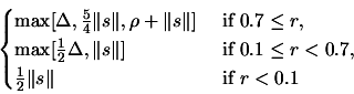 |
(6.3) |
If
 ,
set
,
set
 .
.
- Store
 inside the interpolation dataset:
choose the point
inside the interpolation dataset:
choose the point
 to remove using technique of Section
3.4.3 and replace it by
using the
technique of Section 3.4.4. Let us define the
to remove using technique of Section
3.4.3 and replace it by
using the
technique of Section 3.4.4. Let us define the
- Update the index of the best point in the dataset. Set
![$ F_{new} := \min [ F_{old}, F_{new} ]$](img827.png) .
.
- Update the value of
 which is used during the check of
the validity of the polynomial around
which is used during the check of
the validity of the polynomial around
 (see Section
3.4.1 and more precisely Equation 3.34).
(see Section
3.4.1 and more precisely Equation 3.34).
- If there was an improvement in the quality of the solution
OR if
 OR if
OR if
 then go
back to point 4.
then go
back to point 4.
- Parallel extension: same as point 4.
- We must now check the validity of our model using the
technique of Section 3.4.2. We will need, to check
this validity, a parameter
 : see Section
6.1 to know how to compute it.
: see Section
6.1 to know how to compute it.
- Model is invalid: We will improve the quality of our
model . We will remove the worst point
 of the
dataset and replace it by a better point (we must also update the
value of if a new function evaluation has been made). This
algorithm is described in Section 3.4.2. We will
possibly have to update the index of the best point in the
dataset and . Once this is finished, return to step 4.
of the
dataset and replace it by a better point (we must also update the
value of if a new function evaluation has been made). This
algorithm is described in Section 3.4.2. We will
possibly have to update the index of the best point in the
dataset and . Once this is finished, return to step 4.
- Model is valid If
 return to step 4,
otherwise continue.
return to step 4,
otherwise continue.
- If
 , we have nearly finished the algorithm:
go to step 21, otherwise continue to the next step.
, we have nearly finished the algorithm:
go to step 21, otherwise continue to the next step.
- Update of the global trust region radius.
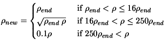 |
(6.4) |
Set
![$ \displaystyle \Delta:=\max[\frac{\rho}{2}, \rho_{new}]$](img832.png) . Set
. Set
 .
.
- Set
 . Apply a
translation of
. Apply a
translation of
 to , to the set of Newton
polynomials
to , to the set of Newton
polynomials  which defines (see Equation 3.26)
and to the whole dataset
. Go
back to step 4.
which defines (see Equation 3.26)
and to the whole dataset
. Go
back to step 4.
- The iteration are now complete but one more value of
may be required before termination. Indeed, we recall from step 6
and step 8 of the algorithm that the value of
 has maybe not been computed. Compute
 .
.
- if
 , the solution of the optimization
problem is
and the value of
, the solution of the optimization
problem is
and the value of  at this
point is .
at this
point is .
- if
 , the solution of the optimization
problem is
, the solution of the optimization
problem is
 and the value of at this
point is .
and the value of at this
point is .
Notice the simplified nature of the trust-region update mechanism
of  (step 16). This is the formal consequence of the
observation that the trust-region radius should not be reduced if
the model has not been guaranteed to be valid in the trust region
(step 16). This is the formal consequence of the
observation that the trust-region radius should not be reduced if
the model has not been guaranteed to be valid in the trust region
 .
.
Subsections
Next: The bound .
Up: Unconstrained Optimization
Previous: About the choice of
Contents
Frank Vanden Berghen
2004-04-19