Next: Remarks about the constrained
Up: Detailed description of the
Previous: The SQP algorithm
Contents
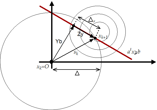
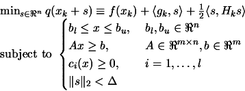
The step  of the constrained algorithm are the solution of:
We will use a null-space, active set approach. We will follow the
notations of section 9.1.1.
- Let
 be a vector of Lagrange Multiplier associated
with all the linear constraints. This vector is recovered from the
previous calculation of the constrained step. Set
be a vector of Lagrange Multiplier associated
with all the linear constraints. This vector is recovered from the
previous calculation of the constrained step. Set  ,
,  The constraints which are active are determined by a
non-null ,
The constraints which are active are determined by a
non-null ,  . If a associated with a
non-linear constraint is not null, set NLActive
. If a associated with a
non-linear constraint is not null, set NLActive ,
otherwise set NLActive
,
otherwise set NLActive .
.
- Compute the matrix
 and
and  associated with the reduced
space of the active box and linear constraints. The active set is
determined by
associated with the reduced
space of the active box and linear constraints. The active set is
determined by  .
.
- We will now compute the step in the reduced-space of
the active box and linear constraints. Check NLActive:
- Compute the Lagrange multipliers
 . If
. If
 for all constraints then terminate. Remove from
the constraints which have negative .
for all constraints then terminate. Remove from
the constraints which have negative .
- Check if a non-linear constraint has been violated. If the
test is true, set NLActive, set
 and go to
(2).
and go to
(2).
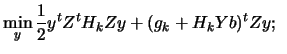
- Solve 9.13 and add if necessary a new box or
linear constraint inside . Set and go to (2).
This is really a small, simple sketch of the implemented
algorithm. The real algorithm has some primitive techniques to
avoid cycling. As you can see, the algorithm is also able to "warm
start", using the previous computed at the previous
step.
Next: Remarks about the constrained
Up: Detailed description of the
Previous: The SQP algorithm
Contents
Frank Vanden Berghen
2004-04-19
 subject to