Next: The constrained step in
Up: Detailed description of the
Previous: The QP algorithm
Contents
Subsections
The material of this section is based on the following references:
[NW99,Fle87,PT93].
The SQP algorithm is:
- set

- Solve the QP subproblem described on equation 8.53
to determine
 and let
 be the vector of
the Lagrange multiplier of the linear constraints obtained from
the QP.
be the vector of
the Lagrange multiplier of the linear constraints obtained from
the QP.
- Compute the length
 of the step and set
- Compute
 from
from  using a quasi-Newton formula
- Increment
 . Stop if
![$ \begin{picture}(.27,.3)
\put(0,0){\makebox(0,0)[bl]{$\nabla$}}
\put(.16,.17){\circle*{.18}}
\end{picture}
\L (x_k,\lambda_k)\approx 0$](img1083.png) . Otherwise, go to step 2.
. Otherwise, go to step 2.
We will now give a detailed discussion of each step. The QP
subproblem has been described in the previous section.
From the QP, we got a direction of research. To have a
more robust code, we will apply the first Wolf condition (see
equation 13.4) which is recalled here:
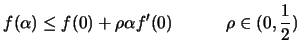 |
(9.18) |
where
 . This condition ensure a
``sufficient enough" reduction of the objective function at each
step. Unfortunately, in the constrained case, sufficient reduction
of the objective function is not enough. We must also ensure
reduction of the infeasibility. Therefore, we will use a modified
form of the first Wolf condition where
. This condition ensure a
``sufficient enough" reduction of the objective function at each
step. Unfortunately, in the constrained case, sufficient reduction
of the objective function is not enough. We must also ensure
reduction of the infeasibility. Therefore, we will use a modified
form of the first Wolf condition where
 and
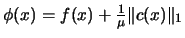
and  is a merit function. We will use in the
optimizer the
is a merit function. We will use in the
optimizer the  merit function:
 |
(9.19) |
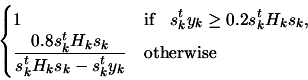
where  is called the penalty parameter. A suitable value for the
penalty parameter is obtained by choosing a constant
is called the penalty parameter. A suitable value for the
penalty parameter is obtained by choosing a constant  and
defining
and
defining  at every iteration too be
 |
(9.20) |
In equation
9.18, we must calculate  : the directional
derivative of
: the directional
derivative of  in the direction at
  :
:
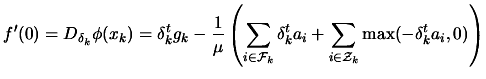 |
(9.21) |
where
 ,
,
 ,
,
 ,
,
 . The algorithm which
computes the length of the step is thus:
. The algorithm which
computes the length of the step is thus:
- Set
 ,
,  current point,
 direction of research
- Test the Wolf condition equation 9.18:
 ?
?
- True: Set
 and go to
step 3.
and go to
step 3.
- False: Set
 and return to the
beginning of step 2.
and return to the
beginning of step 2.
- We have successfully computed the length
 of the step.
Figure 9.5:
Maratos effect.
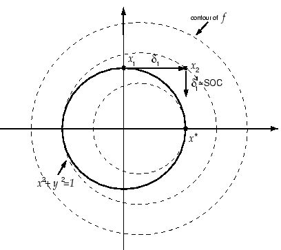 |
The merit function
 can sometimes reject steps (=to give
 ) that are
making good progress towards the solution. This phenomenon is
known as the Maratos effect. It is illustrated by the following
example:
) that are
making good progress towards the solution. This phenomenon is
known as the Maratos effect. It is illustrated by the following
example:
 Subject to Subject to  |
(9.22) |
The optimal solution is
 . The situation is illustrated in figure
9.5. The SQP method moves (
. The situation is illustrated in figure
9.5. The SQP method moves (
 ) from
 to
to
 .
.
In this example, a step
 along the constraint
will always be rejected (
) by
along the constraint
will always be rejected (
) by  merit
function. If no measure are taken, the Maratos effect can
dramatically slow down SQP methods. To avoid the Maratos effect,
we can use a second-order correction step (SOC) in which we
add to a step
merit
function. If no measure are taken, the Maratos effect can
dramatically slow down SQP methods. To avoid the Maratos effect,
we can use a second-order correction step (SOC) in which we
add to a step
 which is computed at
 and which provides sufficient decrease in the
constraints. Another solution is to allow the merit function
to increase on certain iterations (watchdog, non-monotone
strategy).
and which provides sufficient decrease in the
constraints. Another solution is to allow the merit function
to increase on certain iterations (watchdog, non-monotone
strategy).
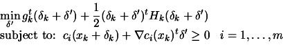
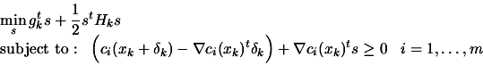
Suppose we have found the SQP step . is the
solution of the following QP problem:
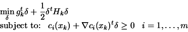 |
(9.23) |
Where we have used a linear
approximation of the constraints at point to find
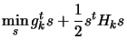
. Suppose this first order approximation of the
constraint is poor. It's better to replace with  ,
the solution of the following problem, where we have used a
quadratical approximation of the constraints:
,
the solution of the following problem, where we have used a
quadratical approximation of the constraints:
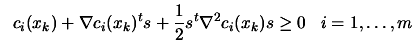
but it's not practical,
even if the hessian of the constraints are individually available,
because the subproblem becomes very hard to solve. Instead, we
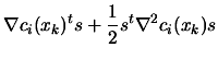
evaluate the constraints at the new point
 and make
use of the following approximation. Ignoring third-order terms, we
have:
and make
use of the following approximation. Ignoring third-order terms, we
have:
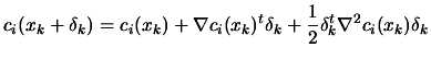 |
(9.26) |
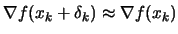
We will assume that, near , we have:
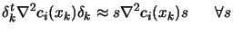 small
small |
(9.27) |
Using 9.27 inside 9.26,
we obtain:
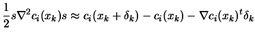 |
(9.28) |
Using 9.28 inside 9.25,
we obtain:
Combining 9.24 and 9.29,
we have:
 |
(9.30) |
Let's define
the solution to problem 9.30. What we really want
is
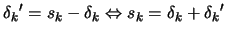 . Using this last equation inside
9.30, we obtain:
is the solution of
. Using this last equation inside
9.30, we obtain:
is the solution of
If we assume that
 (
(
 )(equivalent to assumption
9.27),
we obtain:
)(equivalent to assumption
9.27),
we obtain:
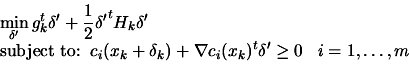 |
(9.31) |
which is similar to the original
equation 9.23 where the constant term of the
constraints are evaluated at
instead of . In
other words, there has been a small shift on the constraints (see
illustration 9.4). We will assume that the active
set of the QP described by 9.23 and the QP
described by 9.31 are the same. Using the notation of
section 9.1.1, we have:
 where where  |
(9.32) |
Where  is the matrix calculated during
the first QP 9.23 which is used to compute
. The SOC step is thus not computationally intensive:
all what we need is an new evaluation of the active constraints at
. The SOC step is illustrated in figure
9.4 and figure 9.5. It's a shift
perpendicular to the active constraints with length proportional
to the amplitude of the violation of the constraints. Using a
classical notation, the SOC step is:
is the matrix calculated during
the first QP 9.23 which is used to compute
. The SOC step is thus not computationally intensive:
all what we need is an new evaluation of the active constraints at
. The SOC step is illustrated in figure
9.4 and figure 9.5. It's a shift
perpendicular to the active constraints with length proportional
to the amplitude of the violation of the constraints. Using a
classical notation, the SOC step is:
 |
(9.33) |
where  is the jacobian matrix
of the active constraints at .
is an approximation of the hessian matrix of the Lagrangian of
the optimization problem.
is the jacobian matrix
of the active constraints at .
is an approximation of the hessian matrix of the Lagrangian of
the optimization problem.
 |
(9.34) |
The QP problem makes the
hypothesis that is definite positive. To obtain a definite
positive approximation of
 we will use the
damped-BFGS updating for SQP (with
we will use the
damped-BFGS updating for SQP (with  ):
):
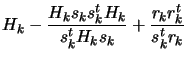
The formula 9.35 is simply the standard BFGS update
formula, with  replaced by
  . It guarantees that
is positive definite.
All the tests are in the form:
. It guarantees that
is positive definite.
All the tests are in the form:
 |
(9.36) |
where  is a residual and
  is a related reference value.
We will stop in the following conditions:
- The length of the step is very small.
- The maximum number of iterations is reached.
- The current point is inside the feasible space, all the
values of
 are positive or null, The step's length is
small.
are positive or null, The step's length is
small.
The SQP algorithm is:
- set
- If termination test is satisfied then stop.
- Solve the QP subproblem described on equation 8.53
to determine and let
be the vector of
the Lagrange multiplier of the linear constraints obtained from
the QP.
- Choose
 such that is a descent direction
for at , using equation 9.20.
such that is a descent direction
for at , using equation 9.20.
- Set
- Test the Wolf condition equation 9.18:
 ?
?
- True: Set
and go to
step 7.
- False: Compute
using equation
9.32
and test:
 ?
?
- True: Set
 and go to step 7.
- False: Set
and go back to the
beginning of step 6.
- Compute from using a quasi-Newton formula
- Increment . Stop if
otherwise, go to step 1.
Next: The constrained step in
Up: Detailed description of the
Previous: The QP algorithm
Contents
Frank Vanden Berghen
2004-04-19