Non-Linear constraints

Penalty Methods

The material of this section is based on the following reference: [Fle87].
Consider the following optimization problem:

$$f(x^*)= \min_x f(x) \; \; c_i(x) \geq 0 , \; i=1,\ldots,m$$ (8.5)

A penalty function is some combination of $f$ and $c$ which enables $f$ to be minimized whilst controlling constraints violations (or near constraints violations) by penalizing them. A primitive penalty function for the inequality constraint problem 8.5 is

$$\phi(x, \sigma)= f(x)+\frac{1}{2} \sigma \sum_{i=1}^{m} [ \min ( c_i(x), 0 )]^2$$ (8.6)

The penalty parameter $\sigma$ increases from iteration to iteration to ensure that the final solution is feasible. The penalty function is thus more and more ill-conditioned (it's more and more difficult to approximate it with a quadratic polynomial). For these reason, penalty function methods are slow. Furthermore, they produce infeasible iterates. Using them for "approach 2" is not possible. However, for "approach 1" they can be a good alternative, especially if the constraints are very non-linear.

Barrier Methods

The material of this section is based on the following references: [NW99,BV04,CGT00f].
Consider the following optimization problem:

$$f(x^*)= \min_x f(x) \; \; c_i(x) \geq 0 , \; i=1,\ldots,m$$ (8.7)

We aggregate the constraints and the objective function in one function which is:

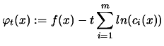$$\varphi_t(x) := f(x) - t \sum_{i=1}^m ln (c_i(x))$$ (8.8)

$t$ is called the barrier parameter. We will refer to $\varphi_t(x)$ as the barrier function. The degree of influence of the barrier term " $- t \sum_{i=1}^m ln (c_i(x))$" is determined by the size of $t$. Under certain conditions $x_t^*$ converges to a local solution $x^*$ of the original problem when $t \rightarrow 0$. Consequently, a strategy for solving the original NLP (Non-Linear Problem) is to solve a sequence of barrier problems for decreasing barrier parameter $t_l$, where $l$ is the counter for the sequence of subproblems. Since the exact solution $$x_{t_l}^*$$ is not of interest for large $t_l$, the corresponding barrier problem is solved only to a relaxed accuracy $\epsilon_l$, and the approximate solution is then used as a starting point for the solution of the next barrier problem. The radius of convergence of Newton's method applied to 8.8 converges to zero as $t \rightarrow 0$. When $t \rightarrow 0$, the barrier function becomes more and more difficult to approximate with a quadratical function. This lead to poor convergence speed for the newton's method. The conjugate gradient (CG) method can still be very effective, especially if good preconditionners are given. The barrier methods have evolved into primal-dual interior point which are faster. The relevance of these methods in the case of the optimization of high computing load objective functions will thus be discussed at the end of the section relative to the primal-dual interior point methods.