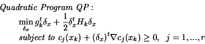
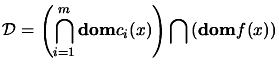
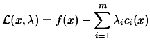
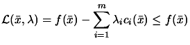
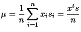
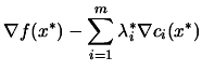
 . We define the
Lagrangian
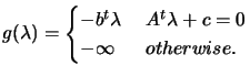
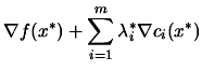
. We define the
Lagrangian
 |
(8.10) |
| (8.11) |
 |
(8.13) |
 |
(8.14) |
| (8.15) |
| (8.17) |
| (8.18) |
 |
(8.19) |
 |
(8.20) |
|
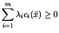
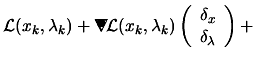
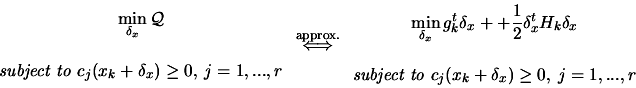
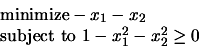
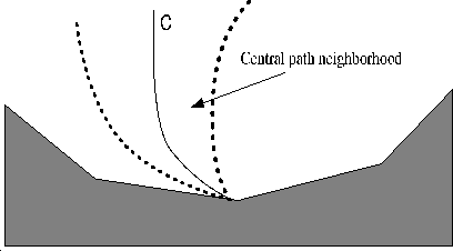
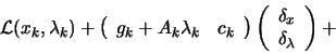
Since the problem is convex, we have (
| |||
 |
|||
 |
|||
![$\displaystyle \left[
\begin{array}{ccc} 0 & A^t & I \\ A & 0 & 0 \\ S & 0 & ...
...rray} \right]=\left[
\begin{array}{c} 0 \\
0 \\ -X S e \end{array} \right]$](img1005.png) |
(8.28) |
| (8.29) |
| (8.30) |
 |
(8.33) |
 |
|||
 |
 or
or
![$\displaystyle W_k=\left[
\begin{array}{cc} H_k & -A_k \\ -A_k & 0 \end{array}...
...\nabla$}}
\put(.16,.17){\circle*{.18}} \end{picture}
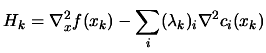
^2 \L (x_k,\lambda_k)] )$](img1072.png) |
(8.50) |
 |
(8.52) |
 |
(8.54) |
| Extrapolated | Multiplier | SQP method | |
| Problem | barrier function | penalty function | (Powell, 1978a) [Pow77] |
| TP1 | 177 | 47 | 6 |
| TP2 | 245 | 172 | 17 |
| TP3 | 123 | 73 | 3 |
![\begin{displaymath}F(x,\lambda,s)= \left[
\begin{array}{c} A^t \lambda +s -c \\ Ax-b \\ X S e \end{array}\right]\end{displaymath}](img997.png)
![$\displaystyle J(x,\lambda, s) \left[ \begin{array}{l} \Delta x \\
\Delta \lambda \\ \Delta s \end{array} \right]= -F(x,\lambda,s)$](img1002.png)
![\begin{displaymath}F(x,\lambda,s)= \left[
\begin{array}{c} A^t \lambda +s -c \\ Ax-b \\ X S e - \tau \end{array}\right]\end{displaymath}](img1014.png)
![$\displaystyle \left[
\begin{array}{ccc} 0 & A^t & I \\ A & 0 & 0 \\ S & 0 & ...
...left[
\begin{array}{c} 0 \\
0 \\ -X S e + \sigma \mu e \end{array} \right]$](img1022.png)
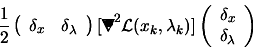
 and
and 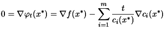

![$\displaystyle \frac{1}{2} \left( \begin{array}{cc} \delta_x & \delta_\lambda
\e...
...\right] \left( \begin{array}{c} \delta_x \\
\delta_\lambda \end{array} \right)$](img1066.png)